Pandas 입문 2
groupby 집중 연습
라이브러리 불러오기
- pandas 라이브러리 불러오고, supermarket_sales.csv 파일 불러오기
- 참고로 미얀마 자료. 얀곤이 옛 수도, 네피도는 현 수도
Pandas 입문 1
판다스
라이브러리 불러오기
1 | import pandas as pd |
1.3.5
테스트
데이터 프레임
1 | temp_dic = {"col1" : [1, 2, 3], |
<class 'pandas.core.frame.DataFrame'>
col1 col2
0 1 3
1 2 4
2 3 5
시리즈
1 | temp_dic = {'a':1, 'b':2, 'c':3} # 인덱스는 숫자나 문자나 모두 가능하다. |
a 1
b 2
c 3
dtype: int64
<class 'pandas.core.series.Series'>
- 언뜻 보기에는 같아보인다.
- 그러나, 다른 클래스고, 메서드도 다르다. 조심해야 한다.
데이터 불러오기
구글 드라이브 연동
Lemonade2016.csv 파일
1 | from google.colab import drive |
Mounted at /content/drive
1 | DATA_PATH = '/content/drive/MyDrive/Colab Notebooks/data/Lemonade2016.csv' |
| Date | Location | Lemon | Orange | Temperature | Leaflets | Price | |
|---|---|---|---|---|---|---|---|
| 0 | 7/1/2016 | Park | 97 | 67 | 70 | 90.0 | 0.25 |
| 1 | 7/2/2016 | Park | 98 | 67 | 72 | 90.0 | 0.25 |
| 2 | 7/3/2016 | Park | 110 | 77 | 71 | 104.0 | 0.25 |
| 3 | 7/4/2016 | Beach | 134 | 99 | 76 | 98.0 | 0.25 |
| 4 | 7/5/2016 | Beach | 159 | 118 | 78 | 135.0 | 0.25 |
| 5 | 7/6/2016 | Beach | 103 | 69 | 82 | 90.0 | 0.25 |
| 6 | 7/6/2016 | Beach | 103 | 69 | 82 | 90.0 | 0.25 |
| 7 | 7/7/2016 | Beach | 143 | 101 | 81 | 135.0 | 0.25 |
| 8 | NaN | Beach | 123 | 86 | 82 | 113.0 | 0.25 |
| 9 | 7/9/2016 | Beach | 134 | 95 | 80 | 126.0 | 0.25 |
| 10 | 7/10/2016 | Beach | 140 | 98 | 82 | 131.0 | 0.25 |
| 11 | 7/11/2016 | Beach | 162 | 120 | 83 | 135.0 | 0.25 |
| 12 | 7/12/2016 | Beach | 130 | 95 | 84 | 99.0 | 0.25 |
| 13 | 7/13/2016 | Beach | 109 | 75 | 77 | 99.0 | 0.25 |
| 14 | 7/14/2016 | Beach | 122 | 85 | 78 | 113.0 | 0.25 |
| 15 | 7/15/2016 | Beach | 98 | 62 | 75 | 108.0 | 0.50 |
| 16 | 7/16/2016 | Beach | 81 | 50 | 74 | 90.0 | 0.50 |
| 17 | 7/17/2016 | Beach | 115 | 76 | 77 | 126.0 | 0.50 |
| 18 | 7/18/2016 | Park | 131 | 92 | 81 | 122.0 | 0.50 |
| 19 | 7/19/2016 | Park | 122 | 85 | 78 | 113.0 | 0.50 |
| 20 | 7/20/2016 | Park | 71 | 42 | 70 | NaN | 0.50 |
| 21 | 7/21/2016 | Park | 83 | 50 | 77 | 90.0 | 0.50 |
| 22 | 7/22/2016 | Park | 112 | 75 | 80 | 108.0 | 0.50 |
| 23 | 7/23/2016 | Park | 120 | 82 | 81 | 117.0 | 0.50 |
| 24 | 7/24/2016 | Park | 121 | 82 | 82 | 117.0 | 0.50 |
| 25 | 7/25/2016 | Park | 156 | 113 | 84 | 135.0 | 0.50 |
| 26 | 7/26/2016 | Park | 176 | 129 | 83 | 158.0 | 0.35 |
| 27 | 7/27/2016 | Park | 104 | 68 | 80 | 99.0 | 0.35 |
| 28 | 7/28/2016 | Park | 96 | 63 | 82 | 90.0 | 0.35 |
| 29 | 7/29/2016 | Park | 100 | 66 | 81 | 95.0 | 0.35 |
| 30 | 7/30/2016 | Beach | 88 | 57 | 82 | 81.0 | 0.35 |
| 31 | 7/31/2016 | Beach | 76 | 47 | 82 | 68.0 | 0.35 |
<script>
const buttonEl =
document.querySelector('#df-377049de-a05e-4731-8fe4-a3adc97f89dd button.colab-df-convert');
buttonEl.style.display =
google.colab.kernel.accessAllowed ? 'block' : 'none';
async function convertToInteractive(key) {
const element = document.querySelector('#df-377049de-a05e-4731-8fe4-a3adc97f89dd');
const dataTable =
await google.colab.kernel.invokeFunction('convertToInteractive',
[key], {});
if (!dataTable) return;
const docLinkHtml = 'Like what you see? Visit the ' +
'<a target="_blank" href=https://colab.research.google.com/notebooks/data_table.ipynb>data table notebook</a>'
+ ' to learn more about interactive tables.';
element.innerHTML = '';
dataTable['output_type'] = 'display_data';
await google.colab.output.renderOutput(dataTable, element);
const docLink = document.createElement('div');
docLink.innerHTML = docLinkHtml;
element.appendChild(docLink);
}
</script>
</div>
- 데이터를 불러왔다. 데이터프레임 메서드를 하나씩 해볼 것이다.
- 첫번째 파악해야 하는 것
- 데이터 구조
1 | juice.info() |
<class 'pandas.core.frame.DataFrame'>
RangeIndex: 32 entries, 0 to 31
Data columns (total 7 columns):
# Column Non-Null Count Dtype
--- ------ -------------- -----
0 Date 31 non-null object
1 Location 32 non-null object
2 Lemon 32 non-null int64
3 Orange 32 non-null int64
4 Temperature 32 non-null int64
5 Leaflets 31 non-null float64
6 Price 32 non-null float64
dtypes: float64(2), int64(3), object(2)
memory usage: 1.9+ KB
- 결측치(NaN)가 있다면 Non-Null Count의 수가 다르다. Date, Leaflets는 결측치가 하나씩 있기 때문에 다른 칼럼에 비해 수가 하나 모자르다. 31.
- .head() 함수는 상위값
- .tail() 함수는 하위값
1 | juice.head() |
| Date | Location | Lemon | Orange | Temperature | Leaflets | Price | |
|---|---|---|---|---|---|---|---|
| 0 | 7/1/2016 | Park | 97 | 67 | 70 | 90.0 | 0.25 |
| 1 | 7/2/2016 | Park | 98 | 67 | 72 | 90.0 | 0.25 |
| 2 | 7/3/2016 | Park | 110 | 77 | 71 | 104.0 | 0.25 |
| 3 | 7/4/2016 | Beach | 134 | 99 | 76 | 98.0 | 0.25 |
| 4 | 7/5/2016 | Beach | 159 | 118 | 78 | 135.0 | 0.25 |
<script>
const buttonEl =
document.querySelector('#df-85ef7723-5da0-4047-9470-852c38d80b3d button.colab-df-convert');
buttonEl.style.display =
google.colab.kernel.accessAllowed ? 'block' : 'none';
async function convertToInteractive(key) {
const element = document.querySelector('#df-85ef7723-5da0-4047-9470-852c38d80b3d');
const dataTable =
await google.colab.kernel.invokeFunction('convertToInteractive',
[key], {});
if (!dataTable) return;
const docLinkHtml = 'Like what you see? Visit the ' +
'<a target="_blank" href=https://colab.research.google.com/notebooks/data_table.ipynb>data table notebook</a>'
+ ' to learn more about interactive tables.';
element.innerHTML = '';
dataTable['output_type'] = 'display_data';
await google.colab.output.renderOutput(dataTable, element);
const docLink = document.createElement('div');
docLink.innerHTML = docLinkHtml;
element.appendChild(docLink);
}
</script>
</div>
1 | juice.tail() |
| Date | Location | Lemon | Orange | Temperature | Leaflets | Price | |
|---|---|---|---|---|---|---|---|
| 27 | 7/27/2016 | Park | 104 | 68 | 80 | 99.0 | 0.35 |
| 28 | 7/28/2016 | Park | 96 | 63 | 82 | 90.0 | 0.35 |
| 29 | 7/29/2016 | Park | 100 | 66 | 81 | 95.0 | 0.35 |
| 30 | 7/30/2016 | Beach | 88 | 57 | 82 | 81.0 | 0.35 |
| 31 | 7/31/2016 | Beach | 76 | 47 | 82 | 68.0 | 0.35 |
<script>
const buttonEl =
document.querySelector('#df-2d82ba80-103f-4ffb-86a3-eb0b3ce806a0 button.colab-df-convert');
buttonEl.style.display =
google.colab.kernel.accessAllowed ? 'block' : 'none';
async function convertToInteractive(key) {
const element = document.querySelector('#df-2d82ba80-103f-4ffb-86a3-eb0b3ce806a0');
const dataTable =
await google.colab.kernel.invokeFunction('convertToInteractive',
[key], {});
if (!dataTable) return;
const docLinkHtml = 'Like what you see? Visit the ' +
'<a target="_blank" href=https://colab.research.google.com/notebooks/data_table.ipynb>data table notebook</a>'
+ ' to learn more about interactive tables.';
element.innerHTML = '';
dataTable['output_type'] = 'display_data';
await google.colab.output.renderOutput(dataTable, element);
const docLink = document.createElement('div');
docLink.innerHTML = docLinkHtml;
element.appendChild(docLink);
}
</script>
</div>
- describe() 함수
- 기술통계량 확인해주는 함수
1 | juice.describe() |
| Lemon | Orange | Temperature | Leaflets | Price | |
|---|---|---|---|---|---|
| count | 32.000000 | 32.000000 | 32.000000 | 31.000000 | 32.000000 |
| mean | 116.156250 | 80.000000 | 78.968750 | 108.548387 | 0.354687 |
| std | 25.823357 | 21.863211 | 4.067847 | 20.117718 | 0.113137 |
| min | 71.000000 | 42.000000 | 70.000000 | 68.000000 | 0.250000 |
| 25% | 98.000000 | 66.750000 | 77.000000 | 90.000000 | 0.250000 |
| 50% | 113.500000 | 76.500000 | 80.500000 | 108.000000 | 0.350000 |
| 75% | 131.750000 | 95.000000 | 82.000000 | 124.000000 | 0.500000 |
| max | 176.000000 | 129.000000 | 84.000000 | 158.000000 | 0.500000 |
<script>
const buttonEl =
document.querySelector('#df-617326f6-852f-40cd-8bdb-9e8c2ac9098d button.colab-df-convert');
buttonEl.style.display =
google.colab.kernel.accessAllowed ? 'block' : 'none';
async function convertToInteractive(key) {
const element = document.querySelector('#df-617326f6-852f-40cd-8bdb-9e8c2ac9098d');
const dataTable =
await google.colab.kernel.invokeFunction('convertToInteractive',
[key], {});
if (!dataTable) return;
const docLinkHtml = 'Like what you see? Visit the ' +
'<a target="_blank" href=https://colab.research.google.com/notebooks/data_table.ipynb>data table notebook</a>'
+ ' to learn more about interactive tables.';
element.innerHTML = '';
dataTable['output_type'] = 'display_data';
await google.colab.output.renderOutput(dataTable, element);
const docLink = document.createElement('div');
docLink.innerHTML = docLinkHtml;
element.appendChild(docLink);
}
</script>
</div>
- Location 칼럼은 문자라서 describe함수가 적용되지 않는다.
- value_counts()
1 | print(juice['Location'].value_counts()) |
Beach 17
Park 15
Name: Location, dtype: int64
<class 'pandas.core.series.Series'>
데이터 다뤄보기
- 행과 열을 만져보자.
- 열 추가(칼럼 추가)
1 | juice['sold'] = 0 # 새로운 컬럼 추가 |
Date Location Lemon Orange Temperature Leaflets Price sold
0 7/1/2016 Park 97 67 70 90.0 0.25 0
1 7/2/2016 Park 98 67 72 90.0 0.25 0
2 7/3/2016 Park 110 77 71 104.0 0.25 0
1 | juice['sold'] = juice['Lemon'] + juice['Orange'] |
Date Location Lemon Orange Temperature Leaflets Price sold
0 7/1/2016 Park 97 67 70 90.0 0.25 164
1 7/2/2016 Park 98 67 72 90.0 0.25 165
2 7/3/2016 Park 110 77 71 104.0 0.25 187
- 퀴즈
- 매출액 = 가격 * 판매량
- Revenue
1 | juice['Revenue'] = juice['Price'] * juice['sold'] |
Date Location Lemon Orange Temperature Leaflets Price sold \
0 7/1/2016 Park 97 67 70 90.0 0.25 164
1 7/2/2016 Park 98 67 72 90.0 0.25 165
2 7/3/2016 Park 110 77 71 104.0 0.25 187
Revenue
0 41.00
1 41.25
2 46.75
- 행과 열 제거
- drop(axis=0, 1)
- axis를 0으로 설정 시, 행(=index) 방향으로 drop() 실행
- axis를 1로 설정 시, 열 방향으로 drop 수행함.
1 | juice_column_drop = juice.drop('sold', axis = 1) # 열 방향, 'sold'열 하나가 통째로 삭제 |
Date Location Lemon Orange Temperature Leaflets Price Revenue
0 7/1/2016 Park 97 67 70 90.0 0.25 41.00
1 7/2/2016 Park 98 67 72 90.0 0.25 41.25
2 7/3/2016 Park 110 77 71 104.0 0.25 46.75
1 | juice_row_drop = juice.drop(0, axis = 0) # 행 방향, 인덱스 0이 통째로 삭제 |
Date Location Lemon Orange Temperature Leaflets Price sold \
1 7/2/2016 Park 98 67 72 90.0 0.25 165
2 7/3/2016 Park 110 77 71 104.0 0.25 187
3 7/4/2016 Beach 134 99 76 98.0 0.25 233
Revenue
1 41.25
2 46.75
3 58.25
데이터 인덱싱
1 | juice[0:5] |
| Date | Location | Lemon | Orange | Temperature | Leaflets | Price | sold | Revenue | |
|---|---|---|---|---|---|---|---|---|---|
| 0 | 7/1/2016 | Park | 97 | 67 | 70 | 90.0 | 0.25 | 164 | 41.00 |
| 1 | 7/2/2016 | Park | 98 | 67 | 72 | 90.0 | 0.25 | 165 | 41.25 |
| 2 | 7/3/2016 | Park | 110 | 77 | 71 | 104.0 | 0.25 | 187 | 46.75 |
| 3 | 7/4/2016 | Beach | 134 | 99 | 76 | 98.0 | 0.25 | 233 | 58.25 |
| 4 | 7/5/2016 | Beach | 159 | 118 | 78 | 135.0 | 0.25 | 277 | 69.25 |
<script>
const buttonEl =
document.querySelector('#df-3ff8756e-ccea-4443-937c-96dd4ef951a2 button.colab-df-convert');
buttonEl.style.display =
google.colab.kernel.accessAllowed ? 'block' : 'none';
async function convertToInteractive(key) {
const element = document.querySelector('#df-3ff8756e-ccea-4443-937c-96dd4ef951a2');
const dataTable =
await google.colab.kernel.invokeFunction('convertToInteractive',
[key], {});
if (!dataTable) return;
const docLinkHtml = 'Like what you see? Visit the ' +
'<a target="_blank" href=https://colab.research.google.com/notebooks/data_table.ipynb>data table notebook</a>'
+ ' to learn more about interactive tables.';
element.innerHTML = '';
dataTable['output_type'] = 'display_data';
await google.colab.output.renderOutput(dataTable, element);
const docLink = document.createElement('div');
docLink.innerHTML = docLinkHtml;
element.appendChild(docLink);
}
</script>
</div>
boolean 값을 활용한 데이터추출
1 | juice['Location'] == "Beach" |
0 False
1 False
2 False
3 True
4 True
5 True
6 True
7 True
8 True
9 True
10 True
11 True
12 True
13 True
14 True
15 True
16 True
17 True
18 False
19 False
20 False
21 False
22 False
23 False
24 False
25 False
26 False
27 False
28 False
29 False
30 True
31 True
Name: Location, dtype: bool
1 | # Location이 Beach인 경우 |
| Date | Location | Lemon | Orange | Temperature | Leaflets | Price | sold | Revenue | |
|---|---|---|---|---|---|---|---|---|---|
| 3 | 7/4/2016 | Beach | 134 | 99 | 76 | 98.0 | 0.25 | 233 | 58.25 |
| 4 | 7/5/2016 | Beach | 159 | 118 | 78 | 135.0 | 0.25 | 277 | 69.25 |
| 5 | 7/6/2016 | Beach | 103 | 69 | 82 | 90.0 | 0.25 | 172 | 43.00 |
| 6 | 7/6/2016 | Beach | 103 | 69 | 82 | 90.0 | 0.25 | 172 | 43.00 |
| 7 | 7/7/2016 | Beach | 143 | 101 | 81 | 135.0 | 0.25 | 244 | 61.00 |
| 8 | NaN | Beach | 123 | 86 | 82 | 113.0 | 0.25 | 209 | 52.25 |
| 9 | 7/9/2016 | Beach | 134 | 95 | 80 | 126.0 | 0.25 | 229 | 57.25 |
| 10 | 7/10/2016 | Beach | 140 | 98 | 82 | 131.0 | 0.25 | 238 | 59.50 |
| 11 | 7/11/2016 | Beach | 162 | 120 | 83 | 135.0 | 0.25 | 282 | 70.50 |
| 12 | 7/12/2016 | Beach | 130 | 95 | 84 | 99.0 | 0.25 | 225 | 56.25 |
| 13 | 7/13/2016 | Beach | 109 | 75 | 77 | 99.0 | 0.25 | 184 | 46.00 |
| 14 | 7/14/2016 | Beach | 122 | 85 | 78 | 113.0 | 0.25 | 207 | 51.75 |
| 15 | 7/15/2016 | Beach | 98 | 62 | 75 | 108.0 | 0.50 | 160 | 80.00 |
| 16 | 7/16/2016 | Beach | 81 | 50 | 74 | 90.0 | 0.50 | 131 | 65.50 |
| 17 | 7/17/2016 | Beach | 115 | 76 | 77 | 126.0 | 0.50 | 191 | 95.50 |
| 30 | 7/30/2016 | Beach | 88 | 57 | 82 | 81.0 | 0.35 | 145 | 50.75 |
| 31 | 7/31/2016 | Beach | 76 | 47 | 82 | 68.0 | 0.35 | 123 | 43.05 |
<script>
const buttonEl =
document.querySelector('#df-f434477b-a70d-4d15-a445-7a178f78849e button.colab-df-convert');
buttonEl.style.display =
google.colab.kernel.accessAllowed ? 'block' : 'none';
async function convertToInteractive(key) {
const element = document.querySelector('#df-f434477b-a70d-4d15-a445-7a178f78849e');
const dataTable =
await google.colab.kernel.invokeFunction('convertToInteractive',
[key], {});
if (!dataTable) return;
const docLinkHtml = 'Like what you see? Visit the ' +
'<a target="_blank" href=https://colab.research.google.com/notebooks/data_table.ipynb>data table notebook</a>'
+ ' to learn more about interactive tables.';
element.innerHTML = '';
dataTable['output_type'] = 'display_data';
await google.colab.output.renderOutput(dataTable, element);
const docLink = document.createElement('div');
docLink.innerHTML = docLinkHtml;
element.appendChild(docLink);
}
</script>
</div>
iloc vs loc
- 차이를 확인한다.
1 | juice.iloc[:, 0:2] # 전체 데이터를 가져와라 그리고 0번부터 1번(n-1) 칼럼을 가져와라 |
| Date | Location | |
|---|---|---|
| 0 | 7/1/2016 | Park |
| 1 | 7/2/2016 | Park |
| 2 | 7/3/2016 | Park |
| 3 | 7/4/2016 | Beach |
| 4 | 7/5/2016 | Beach |
| 5 | 7/6/2016 | Beach |
| 6 | 7/6/2016 | Beach |
| 7 | 7/7/2016 | Beach |
| 8 | NaN | Beach |
| 9 | 7/9/2016 | Beach |
| 10 | 7/10/2016 | Beach |
| 11 | 7/11/2016 | Beach |
| 12 | 7/12/2016 | Beach |
| 13 | 7/13/2016 | Beach |
| 14 | 7/14/2016 | Beach |
| 15 | 7/15/2016 | Beach |
| 16 | 7/16/2016 | Beach |
| 17 | 7/17/2016 | Beach |
| 18 | 7/18/2016 | Park |
| 19 | 7/19/2016 | Park |
| 20 | 7/20/2016 | Park |
| 21 | 7/21/2016 | Park |
| 22 | 7/22/2016 | Park |
| 23 | 7/23/2016 | Park |
| 24 | 7/24/2016 | Park |
| 25 | 7/25/2016 | Park |
| 26 | 7/26/2016 | Park |
| 27 | 7/27/2016 | Park |
| 28 | 7/28/2016 | Park |
| 29 | 7/29/2016 | Park |
| 30 | 7/30/2016 | Beach |
| 31 | 7/31/2016 | Beach |
<script>
const buttonEl =
document.querySelector('#df-d28556da-097b-4c4b-90f3-3548273e5785 button.colab-df-convert');
buttonEl.style.display =
google.colab.kernel.accessAllowed ? 'block' : 'none';
async function convertToInteractive(key) {
const element = document.querySelector('#df-d28556da-097b-4c4b-90f3-3548273e5785');
const dataTable =
await google.colab.kernel.invokeFunction('convertToInteractive',
[key], {});
if (!dataTable) return;
const docLinkHtml = 'Like what you see? Visit the ' +
'<a target="_blank" href=https://colab.research.google.com/notebooks/data_table.ipynb>data table notebook</a>'
+ ' to learn more about interactive tables.';
element.innerHTML = '';
dataTable['output_type'] = 'display_data';
await google.colab.output.renderOutput(dataTable, element);
const docLink = document.createElement('div');
docLink.innerHTML = docLinkHtml;
element.appendChild(docLink);
}
</script>
</div>
1 | %%time |
CPU times: user 735 µs, sys: 0 ns, total: 735 µs
Wall time: 843 µs
| Date | Location | |
|---|---|---|
| 0 | 7/1/2016 | Park |
| 1 | 7/2/2016 | Park |
| 2 | 7/3/2016 | Park |
<script>
const buttonEl =
document.querySelector('#df-3313e9ec-a014-4d12-9209-3fc4ffa27eab button.colab-df-convert');
buttonEl.style.display =
google.colab.kernel.accessAllowed ? 'block' : 'none';
async function convertToInteractive(key) {
const element = document.querySelector('#df-3313e9ec-a014-4d12-9209-3fc4ffa27eab');
const dataTable =
await google.colab.kernel.invokeFunction('convertToInteractive',
[key], {});
if (!dataTable) return;
const docLinkHtml = 'Like what you see? Visit the ' +
'<a target="_blank" href=https://colab.research.google.com/notebooks/data_table.ipynb>data table notebook</a>'
+ ' to learn more about interactive tables.';
element.innerHTML = '';
dataTable['output_type'] = 'display_data';
await google.colab.output.renderOutput(dataTable, element);
const docLink = document.createElement('div');
docLink.innerHTML = docLinkHtml;
element.appendChild(docLink);
}
</script>
</div>
loc
- 라벨 기반
1 | %%time |
CPU times: user 2.58 ms, sys: 0 ns, total: 2.58 ms
Wall time: 6.81 ms
| Date | Location | |
|---|---|---|
| 0 | 7/1/2016 | Park |
| 1 | 7/2/2016 | Park |
| 2 | 7/3/2016 | Park |
<script>
const buttonEl =
document.querySelector('#df-69c0c626-2e18-4cf9-b0b9-4afab44368fd button.colab-df-convert');
buttonEl.style.display =
google.colab.kernel.accessAllowed ? 'block' : 'none';
async function convertToInteractive(key) {
const element = document.querySelector('#df-69c0c626-2e18-4cf9-b0b9-4afab44368fd');
const dataTable =
await google.colab.kernel.invokeFunction('convertToInteractive',
[key], {});
if (!dataTable) return;
const docLinkHtml = 'Like what you see? Visit the ' +
'<a target="_blank" href=https://colab.research.google.com/notebooks/data_table.ipynb>data table notebook</a>'
+ ' to learn more about interactive tables.';
element.innerHTML = '';
dataTable['output_type'] = 'display_data';
await google.colab.output.renderOutput(dataTable, element);
const docLink = document.createElement('div');
docLink.innerHTML = docLinkHtml;
element.appendChild(docLink);
}
</script>
</div>
- iloc가 속도가 빠른 것을 %%time으로 확인 할 수 있다.
컬럼명 별도 추출
- loc만 할 수 있는 기능
1 | juice.loc[juice['Leaflets'] >= 100, ['Date', 'Location']] |
| Date | Location | |
|---|---|---|
| 2 | 7/3/2016 | Park |
| 4 | 7/5/2016 | Beach |
| 7 | 7/7/2016 | Beach |
| 8 | NaN | Beach |
| 9 | 7/9/2016 | Beach |
| 10 | 7/10/2016 | Beach |
| 11 | 7/11/2016 | Beach |
| 14 | 7/14/2016 | Beach |
| 15 | 7/15/2016 | Beach |
| 17 | 7/17/2016 | Beach |
| 18 | 7/18/2016 | Park |
| 19 | 7/19/2016 | Park |
| 22 | 7/22/2016 | Park |
| 23 | 7/23/2016 | Park |
| 24 | 7/24/2016 | Park |
| 25 | 7/25/2016 | Park |
| 26 | 7/26/2016 | Park |
<script>
const buttonEl =
document.querySelector('#df-cce733ce-3a3e-407b-a638-9ea77dfa236f button.colab-df-convert');
buttonEl.style.display =
google.colab.kernel.accessAllowed ? 'block' : 'none';
async function convertToInteractive(key) {
const element = document.querySelector('#df-cce733ce-3a3e-407b-a638-9ea77dfa236f');
const dataTable =
await google.colab.kernel.invokeFunction('convertToInteractive',
[key], {});
if (!dataTable) return;
const docLinkHtml = 'Like what you see? Visit the ' +
'<a target="_blank" href=https://colab.research.google.com/notebooks/data_table.ipynb>data table notebook</a>'
+ ' to learn more about interactive tables.';
element.innerHTML = '';
dataTable['output_type'] = 'display_data';
await google.colab.output.renderOutput(dataTable, element);
const docLink = document.createElement('div');
docLink.innerHTML = docLinkHtml;
element.appendChild(docLink);
}
</script>
</div>
- iloc는 위가 안 된다.
정렬
- sort_values()
1 | juice.sort_values(by=['Revenue'], ascending = False).head() # 내림차순으로 |
| Date | Location | Lemon | Orange | Temperature | Leaflets | Price | sold | Revenue | |
|---|---|---|---|---|---|---|---|---|---|
| 25 | 7/25/2016 | Park | 156 | 113 | 84 | 135.0 | 0.50 | 269 | 134.50 |
| 18 | 7/18/2016 | Park | 131 | 92 | 81 | 122.0 | 0.50 | 223 | 111.50 |
| 26 | 7/26/2016 | Park | 176 | 129 | 83 | 158.0 | 0.35 | 305 | 106.75 |
| 19 | 7/19/2016 | Park | 122 | 85 | 78 | 113.0 | 0.50 | 207 | 103.50 |
| 24 | 7/24/2016 | Park | 121 | 82 | 82 | 117.0 | 0.50 | 203 | 101.50 |
<script>
const buttonEl =
document.querySelector('#df-fdaed60a-bf98-46fe-a701-24e216acb756 button.colab-df-convert');
buttonEl.style.display =
google.colab.kernel.accessAllowed ? 'block' : 'none';
async function convertToInteractive(key) {
const element = document.querySelector('#df-fdaed60a-bf98-46fe-a701-24e216acb756');
const dataTable =
await google.colab.kernel.invokeFunction('convertToInteractive',
[key], {});
if (!dataTable) return;
const docLinkHtml = 'Like what you see? Visit the ' +
'<a target="_blank" href=https://colab.research.google.com/notebooks/data_table.ipynb>data table notebook</a>'
+ ' to learn more about interactive tables.';
element.innerHTML = '';
dataTable['output_type'] = 'display_data';
await google.colab.output.renderOutput(dataTable, element);
const docLink = document.createElement('div');
docLink.innerHTML = docLinkHtml;
element.appendChild(docLink);
}
</script>
</div>
1 | juice2 = juice.sort_values(by=['Price', 'Temperature'], ascending = [False, True]).reset_index(drop=True) |
| Date | Location | Lemon | Orange | Temperature | Leaflets | Price | sold | Revenue | |
|---|---|---|---|---|---|---|---|---|---|
| 0 | 7/20/2016 | Park | 71 | 42 | 70 | NaN | 0.50 | 113 | 56.50 |
| 1 | 7/16/2016 | Beach | 81 | 50 | 74 | 90.0 | 0.50 | 131 | 65.50 |
| 2 | 7/15/2016 | Beach | 98 | 62 | 75 | 108.0 | 0.50 | 160 | 80.00 |
| 3 | 7/17/2016 | Beach | 115 | 76 | 77 | 126.0 | 0.50 | 191 | 95.50 |
| 4 | 7/21/2016 | Park | 83 | 50 | 77 | 90.0 | 0.50 | 133 | 66.50 |
| 5 | 7/19/2016 | Park | 122 | 85 | 78 | 113.0 | 0.50 | 207 | 103.50 |
| 6 | 7/22/2016 | Park | 112 | 75 | 80 | 108.0 | 0.50 | 187 | 93.50 |
| 7 | 7/18/2016 | Park | 131 | 92 | 81 | 122.0 | 0.50 | 223 | 111.50 |
| 8 | 7/23/2016 | Park | 120 | 82 | 81 | 117.0 | 0.50 | 202 | 101.00 |
| 9 | 7/24/2016 | Park | 121 | 82 | 82 | 117.0 | 0.50 | 203 | 101.50 |
| 10 | 7/25/2016 | Park | 156 | 113 | 84 | 135.0 | 0.50 | 269 | 134.50 |
| 11 | 7/27/2016 | Park | 104 | 68 | 80 | 99.0 | 0.35 | 172 | 60.20 |
| 12 | 7/29/2016 | Park | 100 | 66 | 81 | 95.0 | 0.35 | 166 | 58.10 |
| 13 | 7/28/2016 | Park | 96 | 63 | 82 | 90.0 | 0.35 | 159 | 55.65 |
| 14 | 7/30/2016 | Beach | 88 | 57 | 82 | 81.0 | 0.35 | 145 | 50.75 |
| 15 | 7/31/2016 | Beach | 76 | 47 | 82 | 68.0 | 0.35 | 123 | 43.05 |
| 16 | 7/26/2016 | Park | 176 | 129 | 83 | 158.0 | 0.35 | 305 | 106.75 |
| 17 | 7/1/2016 | Park | 97 | 67 | 70 | 90.0 | 0.25 | 164 | 41.00 |
| 18 | 7/3/2016 | Park | 110 | 77 | 71 | 104.0 | 0.25 | 187 | 46.75 |
| 19 | 7/2/2016 | Park | 98 | 67 | 72 | 90.0 | 0.25 | 165 | 41.25 |
| 20 | 7/4/2016 | Beach | 134 | 99 | 76 | 98.0 | 0.25 | 233 | 58.25 |
| 21 | 7/13/2016 | Beach | 109 | 75 | 77 | 99.0 | 0.25 | 184 | 46.00 |
| 22 | 7/5/2016 | Beach | 159 | 118 | 78 | 135.0 | 0.25 | 277 | 69.25 |
| 23 | 7/14/2016 | Beach | 122 | 85 | 78 | 113.0 | 0.25 | 207 | 51.75 |
| 24 | 7/9/2016 | Beach | 134 | 95 | 80 | 126.0 | 0.25 | 229 | 57.25 |
| 25 | 7/7/2016 | Beach | 143 | 101 | 81 | 135.0 | 0.25 | 244 | 61.00 |
| 26 | 7/6/2016 | Beach | 103 | 69 | 82 | 90.0 | 0.25 | 172 | 43.00 |
| 27 | 7/6/2016 | Beach | 103 | 69 | 82 | 90.0 | 0.25 | 172 | 43.00 |
| 28 | NaN | Beach | 123 | 86 | 82 | 113.0 | 0.25 | 209 | 52.25 |
| 29 | 7/10/2016 | Beach | 140 | 98 | 82 | 131.0 | 0.25 | 238 | 59.50 |
| 30 | 7/11/2016 | Beach | 162 | 120 | 83 | 135.0 | 0.25 | 282 | 70.50 |
| 31 | 7/12/2016 | Beach | 130 | 95 | 84 | 99.0 | 0.25 | 225 | 56.25 |
<script>
const buttonEl =
document.querySelector('#df-374e41cd-177f-4906-a3ce-e839f106f7a7 button.colab-df-convert');
buttonEl.style.display =
google.colab.kernel.accessAllowed ? 'block' : 'none';
async function convertToInteractive(key) {
const element = document.querySelector('#df-374e41cd-177f-4906-a3ce-e839f106f7a7');
const dataTable =
await google.colab.kernel.invokeFunction('convertToInteractive',
[key], {});
if (!dataTable) return;
const docLinkHtml = 'Like what you see? Visit the ' +
'<a target="_blank" href=https://colab.research.google.com/notebooks/data_table.ipynb>data table notebook</a>'
+ ' to learn more about interactive tables.';
element.innerHTML = '';
dataTable['output_type'] = 'display_data';
await google.colab.output.renderOutput(dataTable, element);
const docLink = document.createElement('div');
docLink.innerHTML = docLinkHtml;
element.appendChild(docLink);
}
</script>
</div>
Groupby()
- 피벗 테이블을 만드는 것과 똑같음
- 요약하려고
1 | juice.groupby(by = 'Location').count() |
| Date | Lemon | Orange | Temperature | Leaflets | Price | sold | Revenue | |
|---|---|---|---|---|---|---|---|---|
| Location | ||||||||
| Beach | 16 | 17 | 17 | 17 | 17 | 17 | 17 | 17 |
| Park | 15 | 15 | 15 | 15 | 14 | 15 | 15 | 15 |
<script>
const buttonEl =
document.querySelector('#df-9d46cfb2-4ae7-44c5-a9de-d88d60478500 button.colab-df-convert');
buttonEl.style.display =
google.colab.kernel.accessAllowed ? 'block' : 'none';
async function convertToInteractive(key) {
const element = document.querySelector('#df-9d46cfb2-4ae7-44c5-a9de-d88d60478500');
const dataTable =
await google.colab.kernel.invokeFunction('convertToInteractive',
[key], {});
if (!dataTable) return;
const docLinkHtml = 'Like what you see? Visit the ' +
'<a target="_blank" href=https://colab.research.google.com/notebooks/data_table.ipynb>data table notebook</a>'
+ ' to learn more about interactive tables.';
element.innerHTML = '';
dataTable['output_type'] = 'display_data';
await google.colab.output.renderOutput(dataTable, element);
const docLink = document.createElement('div');
docLink.innerHTML = docLinkHtml;
element.appendChild(docLink);
}
</script>
</div>
1 | import numpy as np |
| Revenue | Lemon | |||||||
|---|---|---|---|---|---|---|---|---|
| max | min | sum | mean | max | min | sum | mean | |
| Location | ||||||||
| Beach | 95.5 | 43.0 | 1002.8 | 58.988235 | 162 | 76 | 2020 | 118.823529 |
| Park | 134.5 | 41.0 | 1178.2 | 78.546667 | 176 | 71 | 1697 | 113.133333 |
<script>
const buttonEl =
document.querySelector('#df-d175d024-02cf-46a7-a0ef-d792b2802f03 button.colab-df-convert');
buttonEl.style.display =
google.colab.kernel.accessAllowed ? 'block' : 'none';
async function convertToInteractive(key) {
const element = document.querySelector('#df-d175d024-02cf-46a7-a0ef-d792b2802f03');
const dataTable =
await google.colab.kernel.invokeFunction('convertToInteractive',
[key], {});
if (!dataTable) return;
const docLinkHtml = 'Like what you see? Visit the ' +
'<a target="_blank" href=https://colab.research.google.com/notebooks/data_table.ipynb>data table notebook</a>'
+ ' to learn more about interactive tables.';
element.innerHTML = '';
dataTable['output_type'] = 'display_data';
await google.colab.output.renderOutput(dataTable, element);
const docLink = document.createElement('div');
docLink.innerHTML = docLinkHtml;
element.appendChild(docLink);
}
</script>
</div>
10분 완성 Pandas
Pandas 10분 완성 필사
원본: https://pandas.pydata.org/pandas-docs/stable/user_guide/10min.html
번역본: https://dataitgirls2.github.io/10minutes2pandas/
1 | import pandas as pd |
Object Creation (객체 생성)
- Pandas는 값을 가지고 있는 리스트를 통해 Series를 만들고, 정수로 만들어진 인덱스를 기본값으로 불러올 것입니다.
1 | s = pd.Series([1,3,5,np.nan,6,8]) |
0 1.0
1 3.0
2 5.0
3 NaN
4 6.0
5 8.0
dtype: float64
- datetime 인덱스와 레이블이 있는 열을 가지고 있는 numpy 배열을 전달하여 데이터프레임을 만듭니다.
1 | dates = pd.date_range('20130101', periods=6) |
DatetimeIndex(['2013-01-01', '2013-01-02', '2013-01-03', '2013-01-04',
'2013-01-05', '2013-01-06'],
dtype='datetime64[ns]', freq='D')
1 | df = pd.DataFrame(np.random.randn(6,4), index=dates, columns=list('ABCD')) |
| A | B | C | D | |
|---|---|---|---|---|
| 2013-01-01 | 0.300728 | -0.263258 | 0.231729 | -0.586384 |
| 2013-01-02 | -1.099834 | -1.311782 | 1.250473 | -0.149189 |
| 2013-01-03 | -0.348645 | -0.913132 | 0.087372 | -0.643829 |
| 2013-01-04 | -0.591139 | 1.840492 | 1.067977 | 1.738770 |
| 2013-01-05 | -0.157689 | -0.352707 | -0.331992 | 0.634488 |
| 2013-01-06 | -1.640009 | -0.620559 | -1.613156 | -2.163666 |
<script>
const buttonEl =
document.querySelector('#df-967c470c-7432-4134-a124-707e64036844 button.colab-df-convert');
buttonEl.style.display =
google.colab.kernel.accessAllowed ? 'block' : 'none';
async function convertToInteractive(key) {
const element = document.querySelector('#df-967c470c-7432-4134-a124-707e64036844');
const dataTable =
await google.colab.kernel.invokeFunction('convertToInteractive',
[key], {});
if (!dataTable) return;
const docLinkHtml = 'Like what you see? Visit the ' +
'<a target="_blank" href=https://colab.research.google.com/notebooks/data_table.ipynb>data table notebook</a>'
+ ' to learn more about interactive tables.';
element.innerHTML = '';
dataTable['output_type'] = 'display_data';
await google.colab.output.renderOutput(dataTable, element);
const docLink = document.createElement('div');
docLink.innerHTML = docLinkHtml;
element.appendChild(docLink);
}
</script>
</div>
- Series와 같은 것으로 변환될 수 있는 객체들의 dict로 구성된 데이터프레임을 만듭니다.
1 | df2 = pd.DataFrame({'A' : 1., |
| A | B | C | D | E | F | |
|---|---|---|---|---|---|---|
| 0 | 1.0 | 2013-01-02 | 1.0 | 3 | test | foo |
| 1 | 1.0 | 2013-01-02 | 1.0 | 3 | train | foo |
| 2 | 1.0 | 2013-01-02 | 1.0 | 3 | test | foo |
| 3 | 1.0 | 2013-01-02 | 1.0 | 3 | train | foo |
<script>
const buttonEl =
document.querySelector('#df-7bdbfccf-d22c-4fa9-afaf-b6f9252e8bbf button.colab-df-convert');
buttonEl.style.display =
google.colab.kernel.accessAllowed ? 'block' : 'none';
async function convertToInteractive(key) {
const element = document.querySelector('#df-7bdbfccf-d22c-4fa9-afaf-b6f9252e8bbf');
const dataTable =
await google.colab.kernel.invokeFunction('convertToInteractive',
[key], {});
if (!dataTable) return;
const docLinkHtml = 'Like what you see? Visit the ' +
'<a target="_blank" href=https://colab.research.google.com/notebooks/data_table.ipynb>data table notebook</a>'
+ ' to learn more about interactive tables.';
element.innerHTML = '';
dataTable['output_type'] = 'display_data';
await google.colab.output.renderOutput(dataTable, element);
const docLink = document.createElement('div');
docLink.innerHTML = docLinkHtml;
element.appendChild(docLink);
}
</script>
</div>
- 데이터프레임 결과물의 열은 다양한 데이터 타입 (dtypes)으로 구성됩니다.
1 | df2.dtypes |
A float64
B datetime64[ns]
C float32
D int32
E category
F object
dtype: object
IPython을 이용하고 계시다면 (공용 속성을 포함한) 열 이름에 대한 Tap 자동완성 기능이 자동으로 활성화 됩니다. 다음은 완성될 속성에 대한 부분집합 (subset)입니다.
역자 주 : 아래 제시된 코드의 경우, IPython이 아닌 환경 (Google Colaboratory, Jupyter 등)에서는 사용이 불가능한 코드인 점에 주의하세요.
2. Viewing Data(데이터 확인하기)
1 | print(df.tail(3)) # 끝에서 마지막 3줄을 불러옴 |
A B C D
2013-01-04 -0.591139 1.840492 1.067977 1.738770
2013-01-05 -0.157689 -0.352707 -0.331992 0.634488
2013-01-06 -1.640009 -0.620559 -1.613156 -2.163666
A B C D
2013-01-02 -1.099834 -1.311782 1.250473 -0.149189
2013-01-03 -0.348645 -0.913132 0.087372 -0.643829
2013-01-04 -0.591139 1.840492 1.067977 1.738770
2013-01-05 -0.157689 -0.352707 -0.331992 0.634488
2013-01-06 -1.640009 -0.620559 -1.613156 -2.163666
1 | df.head() # 위에서 5줄 불러옴 |
| A | B | C | D | |
|---|---|---|---|---|
| 2013-01-01 | 0.300728 | -0.263258 | 0.231729 | -0.586384 |
| 2013-01-02 | -1.099834 | -1.311782 | 1.250473 | -0.149189 |
| 2013-01-03 | -0.348645 | -0.913132 | 0.087372 | -0.643829 |
| 2013-01-04 | -0.591139 | 1.840492 | 1.067977 | 1.738770 |
| 2013-01-05 | -0.157689 | -0.352707 | -0.331992 | 0.634488 |
<script>
const buttonEl =
document.querySelector('#df-c8c15f14-8937-456e-80ef-1223b8608eef button.colab-df-convert');
buttonEl.style.display =
google.colab.kernel.accessAllowed ? 'block' : 'none';
async function convertToInteractive(key) {
const element = document.querySelector('#df-c8c15f14-8937-456e-80ef-1223b8608eef');
const dataTable =
await google.colab.kernel.invokeFunction('convertToInteractive',
[key], {});
if (!dataTable) return;
const docLinkHtml = 'Like what you see? Visit the ' +
'<a target="_blank" href=https://colab.research.google.com/notebooks/data_table.ipynb>data table notebook</a>'
+ ' to learn more about interactive tables.';
element.innerHTML = '';
dataTable['output_type'] = 'display_data';
await google.colab.output.renderOutput(dataTable, element);
const docLink = document.createElement('div');
docLink.innerHTML = docLinkHtml;
element.appendChild(docLink);
}
</script>
</div>
- 인덱스 (index), 열 (column) 그리고 numpy 데이터에 대한 세부 정보를 봅니다.
1 | df.index |
DatetimeIndex(['2013-01-01', '2013-01-02', '2013-01-03', '2013-01-04',
'2013-01-05', '2013-01-06'],
dtype='datetime64[ns]', freq='D')
1 | df.columns |
Index(['A', 'B', 'C', 'D'], dtype='object')
1 | df.values |
array([[ 0.30072817, -0.26325765, 0.23172949, -0.58638441],
[-1.09983384, -1.31178153, 1.25047287, -0.14918936],
[-0.3486452 , -0.91313229, 0.08737214, -0.6438286 ],
[-0.59113876, 1.84049219, 1.06797729, 1.73876959],
[-0.15768942, -0.35270749, -0.33199219, 0.6344876 ],
[-1.64000873, -0.62055935, -1.61315579, -2.16366558]])
- describe()는 데이터의 대략적인 통계적 정보 요약을 보여줍니다.
1 | df.describe() |
| A | B | C | D | |
|---|---|---|---|---|
| count | 6.000000 | 6.000000 | 6.000000 | 6.000000 |
| mean | -0.589431 | -0.270158 | 0.115401 | -0.194968 |
| std | 0.692963 | 1.102985 | 1.039055 | 1.316046 |
| min | -1.640009 | -1.311782 | -1.613156 | -2.163666 |
| 25% | -0.972660 | -0.839989 | -0.227151 | -0.629468 |
| 50% | -0.469892 | -0.486633 | 0.159551 | -0.367787 |
| 75% | -0.205428 | -0.285620 | 0.858915 | 0.438568 |
| max | 0.300728 | 1.840492 | 1.250473 | 1.738770 |
<script>
const buttonEl =
document.querySelector('#df-e0954699-6177-4380-af7a-a41cf118eb02 button.colab-df-convert');
buttonEl.style.display =
google.colab.kernel.accessAllowed ? 'block' : 'none';
async function convertToInteractive(key) {
const element = document.querySelector('#df-e0954699-6177-4380-af7a-a41cf118eb02');
const dataTable =
await google.colab.kernel.invokeFunction('convertToInteractive',
[key], {});
if (!dataTable) return;
const docLinkHtml = 'Like what you see? Visit the ' +
'<a target="_blank" href=https://colab.research.google.com/notebooks/data_table.ipynb>data table notebook</a>'
+ ' to learn more about interactive tables.';
element.innerHTML = '';
dataTable['output_type'] = 'display_data';
await google.colab.output.renderOutput(dataTable, element);
const docLink = document.createElement('div');
docLink.innerHTML = docLinkHtml;
element.appendChild(docLink);
}
</script>
</div>
- 데이터를 전치합니다.
1 | df.T |
| 2013-01-01 | 2013-01-02 | 2013-01-03 | 2013-01-04 | 2013-01-05 | 2013-01-06 | |
|---|---|---|---|---|---|---|
| A | 0.300728 | -1.099834 | -0.348645 | -0.591139 | -0.157689 | -1.640009 |
| B | -0.263258 | -1.311782 | -0.913132 | 1.840492 | -0.352707 | -0.620559 |
| C | 0.231729 | 1.250473 | 0.087372 | 1.067977 | -0.331992 | -1.613156 |
| D | -0.586384 | -0.149189 | -0.643829 | 1.738770 | 0.634488 | -2.163666 |
<script>
const buttonEl =
document.querySelector('#df-0bfe1c42-a2e3-45ce-85a6-f9d827483b84 button.colab-df-convert');
buttonEl.style.display =
google.colab.kernel.accessAllowed ? 'block' : 'none';
async function convertToInteractive(key) {
const element = document.querySelector('#df-0bfe1c42-a2e3-45ce-85a6-f9d827483b84');
const dataTable =
await google.colab.kernel.invokeFunction('convertToInteractive',
[key], {});
if (!dataTable) return;
const docLinkHtml = 'Like what you see? Visit the ' +
'<a target="_blank" href=https://colab.research.google.com/notebooks/data_table.ipynb>data table notebook</a>'
+ ' to learn more about interactive tables.';
element.innerHTML = '';
dataTable['output_type'] = 'display_data';
await google.colab.output.renderOutput(dataTable, element);
const docLink = document.createElement('div');
docLink.innerHTML = docLinkHtml;
element.appendChild(docLink);
}
</script>
</div>
- 축 별로 정렬합니다.
1 | df.sort_index(axis=1, ascending=False) |
| D | C | B | A | |
|---|---|---|---|---|
| 2013-01-01 | -0.586384 | 0.231729 | -0.263258 | 0.300728 |
| 2013-01-02 | -0.149189 | 1.250473 | -1.311782 | -1.099834 |
| 2013-01-03 | -0.643829 | 0.087372 | -0.913132 | -0.348645 |
| 2013-01-04 | 1.738770 | 1.067977 | 1.840492 | -0.591139 |
| 2013-01-05 | 0.634488 | -0.331992 | -0.352707 | -0.157689 |
| 2013-01-06 | -2.163666 | -1.613156 | -0.620559 | -1.640009 |
<script>
const buttonEl =
document.querySelector('#df-41da6cb4-f979-4360-b434-78445763e479 button.colab-df-convert');
buttonEl.style.display =
google.colab.kernel.accessAllowed ? 'block' : 'none';
async function convertToInteractive(key) {
const element = document.querySelector('#df-41da6cb4-f979-4360-b434-78445763e479');
const dataTable =
await google.colab.kernel.invokeFunction('convertToInteractive',
[key], {});
if (!dataTable) return;
const docLinkHtml = 'Like what you see? Visit the ' +
'<a target="_blank" href=https://colab.research.google.com/notebooks/data_table.ipynb>data table notebook</a>'
+ ' to learn more about interactive tables.';
element.innerHTML = '';
dataTable['output_type'] = 'display_data';
await google.colab.output.renderOutput(dataTable, element);
const docLink = document.createElement('div');
docLink.innerHTML = docLinkHtml;
element.appendChild(docLink);
}
</script>
</div>
값 별로 정렬합니다.
1 | df.sort_values(by='B') |
| A | B | C | D | |
|---|---|---|---|---|
| 2013-01-02 | -1.099834 | -1.311782 | 1.250473 | -0.149189 |
| 2013-01-03 | -0.348645 | -0.913132 | 0.087372 | -0.643829 |
| 2013-01-06 | -1.640009 | -0.620559 | -1.613156 | -2.163666 |
| 2013-01-05 | -0.157689 | -0.352707 | -0.331992 | 0.634488 |
| 2013-01-01 | 0.300728 | -0.263258 | 0.231729 | -0.586384 |
| 2013-01-04 | -0.591139 | 1.840492 | 1.067977 | 1.738770 |
<script>
const buttonEl =
document.querySelector('#df-f495a21b-27c0-479d-8666-b36c68c7377e button.colab-df-convert');
buttonEl.style.display =
google.colab.kernel.accessAllowed ? 'block' : 'none';
async function convertToInteractive(key) {
const element = document.querySelector('#df-f495a21b-27c0-479d-8666-b36c68c7377e');
const dataTable =
await google.colab.kernel.invokeFunction('convertToInteractive',
[key], {});
if (!dataTable) return;
const docLinkHtml = 'Like what you see? Visit the ' +
'<a target="_blank" href=https://colab.research.google.com/notebooks/data_table.ipynb>data table notebook</a>'
+ ' to learn more about interactive tables.';
element.innerHTML = '';
dataTable['output_type'] = 'display_data';
await google.colab.output.renderOutput(dataTable, element);
const docLink = document.createElement('div');
docLink.innerHTML = docLinkHtml;
element.appendChild(docLink);
}
</script>
</div>
3. Selection(선택)
Getting(데이터 얻기)
- df.A 와 동일한 Series를 생성하는 단일 열을 선택합니다.
1 | df['A'] |
2013-01-01 0.300728
2013-01-02 -1.099834
2013-01-03 -0.348645
2013-01-04 -0.591139
2013-01-05 -0.157689
2013-01-06 -1.640009
Freq: D, Name: A, dtype: float64
- 행을 분할하는 [ ]를 통해 선택합니다.
1 | df[0:3] |
| A | B | C | D | |
|---|---|---|---|---|
| 2013-01-01 | 0.300728 | -0.263258 | 0.231729 | -0.586384 |
| 2013-01-02 | -1.099834 | -1.311782 | 1.250473 | -0.149189 |
| 2013-01-03 | -0.348645 | -0.913132 | 0.087372 | -0.643829 |
<script>
const buttonEl =
document.querySelector('#df-5eddacfa-3ec5-4481-aab9-46338ea6faae button.colab-df-convert');
buttonEl.style.display =
google.colab.kernel.accessAllowed ? 'block' : 'none';
async function convertToInteractive(key) {
const element = document.querySelector('#df-5eddacfa-3ec5-4481-aab9-46338ea6faae');
const dataTable =
await google.colab.kernel.invokeFunction('convertToInteractive',
[key], {});
if (!dataTable) return;
const docLinkHtml = 'Like what you see? Visit the ' +
'<a target="_blank" href=https://colab.research.google.com/notebooks/data_table.ipynb>data table notebook</a>'
+ ' to learn more about interactive tables.';
element.innerHTML = '';
dataTable['output_type'] = 'display_data';
await google.colab.output.renderOutput(dataTable, element);
const docLink = document.createElement('div');
docLink.innerHTML = docLinkHtml;
element.appendChild(docLink);
}
</script>
</div>
1 | df['20130102':'20130104'] |
| A | B | C | D | |
|---|---|---|---|---|
| 2013-01-02 | -1.099834 | -1.311782 | 1.250473 | -0.149189 |
| 2013-01-03 | -0.348645 | -0.913132 | 0.087372 | -0.643829 |
| 2013-01-04 | -0.591139 | 1.840492 | 1.067977 | 1.738770 |
<script>
const buttonEl =
document.querySelector('#df-66eab04d-22d8-4e5a-a15b-72a682ab923c button.colab-df-convert');
buttonEl.style.display =
google.colab.kernel.accessAllowed ? 'block' : 'none';
async function convertToInteractive(key) {
const element = document.querySelector('#df-66eab04d-22d8-4e5a-a15b-72a682ab923c');
const dataTable =
await google.colab.kernel.invokeFunction('convertToInteractive',
[key], {});
if (!dataTable) return;
const docLinkHtml = 'Like what you see? Visit the ' +
'<a target="_blank" href=https://colab.research.google.com/notebooks/data_table.ipynb>data table notebook</a>'
+ ' to learn more about interactive tables.';
element.innerHTML = '';
dataTable['output_type'] = 'display_data';
await google.colab.output.renderOutput(dataTable, element);
const docLink = document.createElement('div');
docLink.innerHTML = docLinkHtml;
element.appendChild(docLink);
}
</script>
</div>
Selection by Label (label을 통한 선택)
1 | df.loc[dates[0]] |
A 0.300728
B -0.263258
C 0.231729
D -0.586384
Name: 2013-01-01 00:00:00, dtype: float64
- 라벨을 사용하여 여러 축 (의 데이터)을 얻습니다.
1 | df.loc[:, ['A','B']] |
| A | B | |
|---|---|---|
| 2013-01-01 | 0.300728 | -0.263258 |
| 2013-01-02 | -1.099834 | -1.311782 |
| 2013-01-03 | -0.348645 | -0.913132 |
| 2013-01-04 | -0.591139 | 1.840492 |
| 2013-01-05 | -0.157689 | -0.352707 |
| 2013-01-06 | -1.640009 | -0.620559 |
<script>
const buttonEl =
document.querySelector('#df-57d0309b-fbf8-4929-b398-0d60d67063ee button.colab-df-convert');
buttonEl.style.display =
google.colab.kernel.accessAllowed ? 'block' : 'none';
async function convertToInteractive(key) {
const element = document.querySelector('#df-57d0309b-fbf8-4929-b398-0d60d67063ee');
const dataTable =
await google.colab.kernel.invokeFunction('convertToInteractive',
[key], {});
if (!dataTable) return;
const docLinkHtml = 'Like what you see? Visit the ' +
'<a target="_blank" href=https://colab.research.google.com/notebooks/data_table.ipynb>data table notebook</a>'
+ ' to learn more about interactive tables.';
element.innerHTML = '';
dataTable['output_type'] = 'display_data';
await google.colab.output.renderOutput(dataTable, element);
const docLink = document.createElement('div');
docLink.innerHTML = docLinkHtml;
element.appendChild(docLink);
}
</script>
</div>
- 양쪽 종단점을 포함한 라벨 슬라이싱을 봅니다.
1 | df.loc['20130102':'20130104', ['A','B']] |
| A | B | |
|---|---|---|
| 2013-01-02 | -1.099834 | -1.311782 |
| 2013-01-03 | -0.348645 | -0.913132 |
| 2013-01-04 | -0.591139 | 1.840492 |
<script>
const buttonEl =
document.querySelector('#df-efba182b-23cd-4e19-bcb3-737481b2322b button.colab-df-convert');
buttonEl.style.display =
google.colab.kernel.accessAllowed ? 'block' : 'none';
async function convertToInteractive(key) {
const element = document.querySelector('#df-efba182b-23cd-4e19-bcb3-737481b2322b');
const dataTable =
await google.colab.kernel.invokeFunction('convertToInteractive',
[key], {});
if (!dataTable) return;
const docLinkHtml = 'Like what you see? Visit the ' +
'<a target="_blank" href=https://colab.research.google.com/notebooks/data_table.ipynb>data table notebook</a>'
+ ' to learn more about interactive tables.';
element.innerHTML = '';
dataTable['output_type'] = 'display_data';
await google.colab.output.renderOutput(dataTable, element);
const docLink = document.createElement('div');
docLink.innerHTML = docLinkHtml;
element.appendChild(docLink);
}
</script>
</div>
- 반환되는 객체의 차원를 줄입니다.
1 | df.loc['20130102',['A','B']] |
A -1.099834
B -1.311782
Name: 2013-01-02 00:00:00, dtype: float64
- 스칼라 값을 얻습니다.
1 | df.loc[dates[0],'A'] |
0.30072817102461075
- 스칼라 값을 더 빠르게 구하는 방법입니다 (앞선 메소드와 동일합니다).
1 | df.at[dates[0], 'A'] |
0.30072817102461075
Selection by Position(위치로 선택하기)
- 넘겨받은 정수의 위치를 기준으로 선택합니다.
1 | df.iloc[3] |
A -0.591139
B 1.840492
C 1.067977
D 1.738770
Name: 2013-01-04 00:00:00, dtype: float64
- 정수로 표기된 슬라이스들을 통해, numpy / python과 유사하게 작동합니다.
1 | df.iloc[3:5,0:2] |
| A | B | |
|---|---|---|
| 2013-01-04 | -0.591139 | 1.840492 |
| 2013-01-05 | -0.157689 | -0.352707 |
<script>
const buttonEl =
document.querySelector('#df-c542aa0e-249b-4629-a46b-89bdb9af6fed button.colab-df-convert');
buttonEl.style.display =
google.colab.kernel.accessAllowed ? 'block' : 'none';
async function convertToInteractive(key) {
const element = document.querySelector('#df-c542aa0e-249b-4629-a46b-89bdb9af6fed');
const dataTable =
await google.colab.kernel.invokeFunction('convertToInteractive',
[key], {});
if (!dataTable) return;
const docLinkHtml = 'Like what you see? Visit the ' +
'<a target="_blank" href=https://colab.research.google.com/notebooks/data_table.ipynb>data table notebook</a>'
+ ' to learn more about interactive tables.';
element.innerHTML = '';
dataTable['output_type'] = 'display_data';
await google.colab.output.renderOutput(dataTable, element);
const docLink = document.createElement('div');
docLink.innerHTML = docLinkHtml;
element.appendChild(docLink);
}
</script>
</div>
- 정수로 표기된 위치값의 리스트들을 통해, numpy / python의 스타일과 유사해집니다.
1 | df.iloc[[1,2,4],[0,2]] |
| A | C | |
|---|---|---|
| 2013-01-02 | -1.099834 | 1.250473 |
| 2013-01-03 | -0.348645 | 0.087372 |
| 2013-01-05 | -0.157689 | -0.331992 |
<script>
const buttonEl =
document.querySelector('#df-55d5daf9-c009-4d79-b075-b29d55365755 button.colab-df-convert');
buttonEl.style.display =
google.colab.kernel.accessAllowed ? 'block' : 'none';
async function convertToInteractive(key) {
const element = document.querySelector('#df-55d5daf9-c009-4d79-b075-b29d55365755');
const dataTable =
await google.colab.kernel.invokeFunction('convertToInteractive',
[key], {});
if (!dataTable) return;
const docLinkHtml = 'Like what you see? Visit the ' +
'<a target="_blank" href=https://colab.research.google.com/notebooks/data_table.ipynb>data table notebook</a>'
+ ' to learn more about interactive tables.';
element.innerHTML = '';
dataTable['output_type'] = 'display_data';
await google.colab.output.renderOutput(dataTable, element);
const docLink = document.createElement('div');
docLink.innerHTML = docLinkHtml;
element.appendChild(docLink);
}
</script>
</div>
- 명시적으로 행을 나누고자 하는 경우입니다.
1 | df.iloc[1:3,:] |
| A | B | C | D | |
|---|---|---|---|---|
| 2013-01-02 | -1.099834 | -1.311782 | 1.250473 | -0.149189 |
| 2013-01-03 | -0.348645 | -0.913132 | 0.087372 | -0.643829 |
<script>
const buttonEl =
document.querySelector('#df-71b47cbb-5679-42a1-a3c2-9a4c0d93c913 button.colab-df-convert');
buttonEl.style.display =
google.colab.kernel.accessAllowed ? 'block' : 'none';
async function convertToInteractive(key) {
const element = document.querySelector('#df-71b47cbb-5679-42a1-a3c2-9a4c0d93c913');
const dataTable =
await google.colab.kernel.invokeFunction('convertToInteractive',
[key], {});
if (!dataTable) return;
const docLinkHtml = 'Like what you see? Visit the ' +
'<a target="_blank" href=https://colab.research.google.com/notebooks/data_table.ipynb>data table notebook</a>'
+ ' to learn more about interactive tables.';
element.innerHTML = '';
dataTable['output_type'] = 'display_data';
await google.colab.output.renderOutput(dataTable, element);
const docLink = document.createElement('div');
docLink.innerHTML = docLinkHtml;
element.appendChild(docLink);
}
</script>
</div>
- 명시적으로 열을 나누고자 하는 경우입니다.
1 | df.iloc[:,1:3] |
| B | C | |
|---|---|---|
| 2013-01-01 | -0.263258 | 0.231729 |
| 2013-01-02 | -1.311782 | 1.250473 |
| 2013-01-03 | -0.913132 | 0.087372 |
| 2013-01-04 | 1.840492 | 1.067977 |
| 2013-01-05 | -0.352707 | -0.331992 |
| 2013-01-06 | -0.620559 | -1.613156 |
<script>
const buttonEl =
document.querySelector('#df-9754adb0-b2e1-418c-b56a-aeac9f8649ee button.colab-df-convert');
buttonEl.style.display =
google.colab.kernel.accessAllowed ? 'block' : 'none';
async function convertToInteractive(key) {
const element = document.querySelector('#df-9754adb0-b2e1-418c-b56a-aeac9f8649ee');
const dataTable =
await google.colab.kernel.invokeFunction('convertToInteractive',
[key], {});
if (!dataTable) return;
const docLinkHtml = 'Like what you see? Visit the ' +
'<a target="_blank" href=https://colab.research.google.com/notebooks/data_table.ipynb>data table notebook</a>'
+ ' to learn more about interactive tables.';
element.innerHTML = '';
dataTable['output_type'] = 'display_data';
await google.colab.output.renderOutput(dataTable, element);
const docLink = document.createElement('div');
docLink.innerHTML = docLinkHtml;
element.appendChild(docLink);
}
</script>
</div>
- 명시적으로 (특정한) 값을 얻고자 하는 경우입니다.
1 | df.iloc[1,1] |
-1.311781527749884
- 스칼라 값을 빠르게 얻는 방법입니다 (위의 방식과 동일합니다).
1 | df.iat[1,1] |
-1.311781527749884
Boolean Indexing
- 데이터를 선택하기 위해 단일 열의 값을 사용합니다.
1 | df[df.A > 0] |
| A | B | C | D | |
|---|---|---|---|---|
| 2013-01-01 | 0.300728 | -0.263258 | 0.231729 | -0.586384 |
<script>
const buttonEl =
document.querySelector('#df-16044eaf-c404-4801-9af5-c6041cce22c2 button.colab-df-convert');
buttonEl.style.display =
google.colab.kernel.accessAllowed ? 'block' : 'none';
async function convertToInteractive(key) {
const element = document.querySelector('#df-16044eaf-c404-4801-9af5-c6041cce22c2');
const dataTable =
await google.colab.kernel.invokeFunction('convertToInteractive',
[key], {});
if (!dataTable) return;
const docLinkHtml = 'Like what you see? Visit the ' +
'<a target="_blank" href=https://colab.research.google.com/notebooks/data_table.ipynb>data table notebook</a>'
+ ' to learn more about interactive tables.';
element.innerHTML = '';
dataTable['output_type'] = 'display_data';
await google.colab.output.renderOutput(dataTable, element);
const docLink = document.createElement('div');
docLink.innerHTML = docLinkHtml;
element.appendChild(docLink);
}
</script>
</div>
- Boolean 조건을 충족하는 데이터프레임에서 값을 선택합니다.
1 | df[df > 0] |
| A | B | C | D | |
|---|---|---|---|---|
| 2013-01-01 | 0.300728 | NaN | 0.231729 | NaN |
| 2013-01-02 | NaN | NaN | 1.250473 | NaN |
| 2013-01-03 | NaN | NaN | 0.087372 | NaN |
| 2013-01-04 | NaN | 1.840492 | 1.067977 | 1.738770 |
| 2013-01-05 | NaN | NaN | NaN | 0.634488 |
| 2013-01-06 | NaN | NaN | NaN | NaN |
<script>
const buttonEl =
document.querySelector('#df-31e35218-2394-43e7-bc03-233c098097df button.colab-df-convert');
buttonEl.style.display =
google.colab.kernel.accessAllowed ? 'block' : 'none';
async function convertToInteractive(key) {
const element = document.querySelector('#df-31e35218-2394-43e7-bc03-233c098097df');
const dataTable =
await google.colab.kernel.invokeFunction('convertToInteractive',
[key], {});
if (!dataTable) return;
const docLinkHtml = 'Like what you see? Visit the ' +
'<a target="_blank" href=https://colab.research.google.com/notebooks/data_table.ipynb>data table notebook</a>'
+ ' to learn more about interactive tables.';
element.innerHTML = '';
dataTable['output_type'] = 'display_data';
await google.colab.output.renderOutput(dataTable, element);
const docLink = document.createElement('div');
docLink.innerHTML = docLinkHtml;
element.appendChild(docLink);
}
</script>
</div>
- 필터링을 위한 메소드 isin()을 사용합니다.
1 | df2 = df.copy() |
1 | df2['E'] = ['one', 'one', 'two', 'three', 'four', 'three'] |
| A | B | C | D | E | |
|---|---|---|---|---|---|
| 2013-01-01 | 0.300728 | -0.263258 | 0.231729 | -0.586384 | one |
| 2013-01-02 | -1.099834 | -1.311782 | 1.250473 | -0.149189 | one |
| 2013-01-03 | -0.348645 | -0.913132 | 0.087372 | -0.643829 | two |
| 2013-01-04 | -0.591139 | 1.840492 | 1.067977 | 1.738770 | three |
| 2013-01-05 | -0.157689 | -0.352707 | -0.331992 | 0.634488 | four |
| 2013-01-06 | -1.640009 | -0.620559 | -1.613156 | -2.163666 | three |
<script>
const buttonEl =
document.querySelector('#df-332f267a-157c-4418-b60d-3d784156a52c button.colab-df-convert');
buttonEl.style.display =
google.colab.kernel.accessAllowed ? 'block' : 'none';
async function convertToInteractive(key) {
const element = document.querySelector('#df-332f267a-157c-4418-b60d-3d784156a52c');
const dataTable =
await google.colab.kernel.invokeFunction('convertToInteractive',
[key], {});
if (!dataTable) return;
const docLinkHtml = 'Like what you see? Visit the ' +
'<a target="_blank" href=https://colab.research.google.com/notebooks/data_table.ipynb>data table notebook</a>'
+ ' to learn more about interactive tables.';
element.innerHTML = '';
dataTable['output_type'] = 'display_data';
await google.colab.output.renderOutput(dataTable, element);
const docLink = document.createElement('div');
docLink.innerHTML = docLinkHtml;
element.appendChild(docLink);
}
</script>
</div>
1 | df2[df2['E'].isin(['two','four'])] |
| A | B | C | D | E | |
|---|---|---|---|---|---|
| 2013-01-03 | -0.348645 | -0.913132 | 0.087372 | -0.643829 | two |
| 2013-01-05 | -0.157689 | -0.352707 | -0.331992 | 0.634488 | four |
<script>
const buttonEl =
document.querySelector('#df-b0d3f1bc-76c3-42fa-80ac-b8f6838eae60 button.colab-df-convert');
buttonEl.style.display =
google.colab.kernel.accessAllowed ? 'block' : 'none';
async function convertToInteractive(key) {
const element = document.querySelector('#df-b0d3f1bc-76c3-42fa-80ac-b8f6838eae60');
const dataTable =
await google.colab.kernel.invokeFunction('convertToInteractive',
[key], {});
if (!dataTable) return;
const docLinkHtml = 'Like what you see? Visit the ' +
'<a target="_blank" href=https://colab.research.google.com/notebooks/data_table.ipynb>data table notebook</a>'
+ ' to learn more about interactive tables.';
element.innerHTML = '';
dataTable['output_type'] = 'display_data';
await google.colab.output.renderOutput(dataTable, element);
const docLink = document.createElement('div');
docLink.innerHTML = docLinkHtml;
element.appendChild(docLink);
}
</script>
</div>
setting(설정)
- 새 열을 설정하면 데이터가 인덱스 별로 자동 정렬됩니다.
1 | s1 = pd.Series([1,2,3,4,5,6], index=pd.date_range('20130102', periods=6)) |
2013-01-02 1
2013-01-03 2
2013-01-04 3
2013-01-05 4
2013-01-06 5
2013-01-07 6
Freq: D, dtype: int64
1 | df['F'] = s1 |
- 라벨에 의해 값을 설정합니다.
1 | df.at[dates[0],'A'] = 0 |
- 위치에 의해 값을 설정합니다.
1 | df.iat[0,1] = 0 |
- Numpy 배열을 사용한 할당에 의해 값을 설정합니다.
1 | df.loc[:, 'D'] = np.array([5] * len(df)) |
| A | B | C | D | F | |
|---|---|---|---|---|---|
| 2013-01-01 | 0.000000 | 0.000000 | 0.231729 | 5 | NaN |
| 2013-01-02 | -1.099834 | -1.311782 | 1.250473 | 5 | 1.0 |
| 2013-01-03 | -0.348645 | -0.913132 | 0.087372 | 5 | 2.0 |
| 2013-01-04 | -0.591139 | 1.840492 | 1.067977 | 5 | 3.0 |
| 2013-01-05 | -0.157689 | -0.352707 | -0.331992 | 5 | 4.0 |
| 2013-01-06 | -1.640009 | -0.620559 | -1.613156 | 5 | 5.0 |
<script>
const buttonEl =
document.querySelector('#df-53de9a37-f969-4912-ac04-86a4cc6f332b button.colab-df-convert');
buttonEl.style.display =
google.colab.kernel.accessAllowed ? 'block' : 'none';
async function convertToInteractive(key) {
const element = document.querySelector('#df-53de9a37-f969-4912-ac04-86a4cc6f332b');
const dataTable =
await google.colab.kernel.invokeFunction('convertToInteractive',
[key], {});
if (!dataTable) return;
const docLinkHtml = 'Like what you see? Visit the ' +
'<a target="_blank" href=https://colab.research.google.com/notebooks/data_table.ipynb>data table notebook</a>'
+ ' to learn more about interactive tables.';
element.innerHTML = '';
dataTable['output_type'] = 'display_data';
await google.colab.output.renderOutput(dataTable, element);
const docLink = document.createElement('div');
docLink.innerHTML = docLinkHtml;
element.appendChild(docLink);
}
</script>
</div>
- where 연산을 설정합니다.
1 | df2 = df.copy() |
1 | df2[df2 > 0] = -df2 |
| A | B | C | D | F | |
|---|---|---|---|---|---|
| 2013-01-01 | 0.000000 | 0.000000 | -0.231729 | -5 | NaN |
| 2013-01-02 | -1.099834 | -1.311782 | -1.250473 | -5 | -1.0 |
| 2013-01-03 | -0.348645 | -0.913132 | -0.087372 | -5 | -2.0 |
| 2013-01-04 | -0.591139 | -1.840492 | -1.067977 | -5 | -3.0 |
| 2013-01-05 | -0.157689 | -0.352707 | -0.331992 | -5 | -4.0 |
| 2013-01-06 | -1.640009 | -0.620559 | -1.613156 | -5 | -5.0 |
<script>
const buttonEl =
document.querySelector('#df-6b2a97e6-7a40-4d52-b4b0-11fa99013880 button.colab-df-convert');
buttonEl.style.display =
google.colab.kernel.accessAllowed ? 'block' : 'none';
async function convertToInteractive(key) {
const element = document.querySelector('#df-6b2a97e6-7a40-4d52-b4b0-11fa99013880');
const dataTable =
await google.colab.kernel.invokeFunction('convertToInteractive',
[key], {});
if (!dataTable) return;
const docLinkHtml = 'Like what you see? Visit the ' +
'<a target="_blank" href=https://colab.research.google.com/notebooks/data_table.ipynb>data table notebook</a>'
+ ' to learn more about interactive tables.';
element.innerHTML = '';
dataTable['output_type'] = 'display_data';
await google.colab.output.renderOutput(dataTable, element);
const docLink = document.createElement('div');
docLink.innerHTML = docLinkHtml;
element.appendChild(docLink);
}
</script>
</div>
Missing Data(결측치)
- Pandas는 결측치를 표현하기 위해 주로 np.nan 값을 사용합니다.
- Reindexing으로 지정된 축 상의 인덱스를 변경 / 추가 / 삭제할 수 있습니다. Reindexing은 데이터의 복사본을 반환합니다.
1 | df1 = df.reindex(index=dates[0:4], columns=list(df.columns) + ['E']) |
1 | df1.loc[dates[0]:dates[1], 'E'] =1 |
| A | B | C | D | F | E | |
|---|---|---|---|---|---|---|
| 2013-01-01 | 0.000000 | 0.000000 | 0.231729 | 5 | NaN | 1.0 |
| 2013-01-02 | -1.099834 | -1.311782 | 1.250473 | 5 | 1.0 | 1.0 |
| 2013-01-03 | -0.348645 | -0.913132 | 0.087372 | 5 | 2.0 | NaN |
| 2013-01-04 | -0.591139 | 1.840492 | 1.067977 | 5 | 3.0 | NaN |
<script>
const buttonEl =
document.querySelector('#df-854eff28-d5c6-493e-9c56-3d573cd836da button.colab-df-convert');
buttonEl.style.display =
google.colab.kernel.accessAllowed ? 'block' : 'none';
async function convertToInteractive(key) {
const element = document.querySelector('#df-854eff28-d5c6-493e-9c56-3d573cd836da');
const dataTable =
await google.colab.kernel.invokeFunction('convertToInteractive',
[key], {});
if (!dataTable) return;
const docLinkHtml = 'Like what you see? Visit the ' +
'<a target="_blank" href=https://colab.research.google.com/notebooks/data_table.ipynb>data table notebook</a>'
+ ' to learn more about interactive tables.';
element.innerHTML = '';
dataTable['output_type'] = 'display_data';
await google.colab.output.renderOutput(dataTable, element);
const docLink = document.createElement('div');
docLink.innerHTML = docLinkHtml;
element.appendChild(docLink);
}
</script>
</div>
- 결측치를 가지고 있는 행들을 지웁니다.
1 | df1.dropna(how='any') |
| A | B | C | D | F | E | |
|---|---|---|---|---|---|---|
| 2013-01-02 | -1.099834 | -1.311782 | 1.250473 | 5 | 1.0 | 1.0 |
<script>
const buttonEl =
document.querySelector('#df-9a8f93a0-529a-45d2-9bc3-6a5becc0ae58 button.colab-df-convert');
buttonEl.style.display =
google.colab.kernel.accessAllowed ? 'block' : 'none';
async function convertToInteractive(key) {
const element = document.querySelector('#df-9a8f93a0-529a-45d2-9bc3-6a5becc0ae58');
const dataTable =
await google.colab.kernel.invokeFunction('convertToInteractive',
[key], {});
if (!dataTable) return;
const docLinkHtml = 'Like what you see? Visit the ' +
'<a target="_blank" href=https://colab.research.google.com/notebooks/data_table.ipynb>data table notebook</a>'
+ ' to learn more about interactive tables.';
element.innerHTML = '';
dataTable['output_type'] = 'display_data';
await google.colab.output.renderOutput(dataTable, element);
const docLink = document.createElement('div');
docLink.innerHTML = docLinkHtml;
element.appendChild(docLink);
}
</script>
</div>
- 결측치를 채워 넣습니다.
1 | df1.fillna(value=5) # 5로 채워넣기 |
| A | B | C | D | F | E | |
|---|---|---|---|---|---|---|
| 2013-01-01 | 0.000000 | 0.000000 | 0.231729 | 5 | 5.0 | 1.0 |
| 2013-01-02 | -1.099834 | -1.311782 | 1.250473 | 5 | 1.0 | 1.0 |
| 2013-01-03 | -0.348645 | -0.913132 | 0.087372 | 5 | 2.0 | 5.0 |
| 2013-01-04 | -0.591139 | 1.840492 | 1.067977 | 5 | 3.0 | 5.0 |
<script>
const buttonEl =
document.querySelector('#df-15ea5efe-2279-441d-917a-153c8e4accb6 button.colab-df-convert');
buttonEl.style.display =
google.colab.kernel.accessAllowed ? 'block' : 'none';
async function convertToInteractive(key) {
const element = document.querySelector('#df-15ea5efe-2279-441d-917a-153c8e4accb6');
const dataTable =
await google.colab.kernel.invokeFunction('convertToInteractive',
[key], {});
if (!dataTable) return;
const docLinkHtml = 'Like what you see? Visit the ' +
'<a target="_blank" href=https://colab.research.google.com/notebooks/data_table.ipynb>data table notebook</a>'
+ ' to learn more about interactive tables.';
element.innerHTML = '';
dataTable['output_type'] = 'display_data';
await google.colab.output.renderOutput(dataTable, element);
const docLink = document.createElement('div');
docLink.innerHTML = docLinkHtml;
element.appendChild(docLink);
}
</script>
</div>
- nan인 값에 boolean을 통한 표식을 얻습니다.
- 역자 주 : 데이터프레임의 모든 값이 boolean 형태로 표시되도록 하며, nan인 값에만 True가 표시되게 하는 함수입니다.
1 | pd.isna(df1) |
| A | B | C | D | F | E | |
|---|---|---|---|---|---|---|
| 2013-01-01 | False | False | False | False | True | False |
| 2013-01-02 | False | False | False | False | False | False |
| 2013-01-03 | False | False | False | False | False | True |
| 2013-01-04 | False | False | False | False | False | True |
<script>
const buttonEl =
document.querySelector('#df-17e39b79-8d76-47c6-8375-a8f56909c185 button.colab-df-convert');
buttonEl.style.display =
google.colab.kernel.accessAllowed ? 'block' : 'none';
async function convertToInteractive(key) {
const element = document.querySelector('#df-17e39b79-8d76-47c6-8375-a8f56909c185');
const dataTable =
await google.colab.kernel.invokeFunction('convertToInteractive',
[key], {});
if (!dataTable) return;
const docLinkHtml = 'Like what you see? Visit the ' +
'<a target="_blank" href=https://colab.research.google.com/notebooks/data_table.ipynb>data table notebook</a>'
+ ' to learn more about interactive tables.';
element.innerHTML = '';
dataTable['output_type'] = 'display_data';
await google.colab.output.renderOutput(dataTable, element);
const docLink = document.createElement('div');
docLink.innerHTML = docLinkHtml;
element.appendChild(docLink);
}
</script>
</div>
Operation (연산)
stats (통계)
일반적으로 결측치를 제외한 후 연산됩니다.
기술통계를 수행합니다.
1 | df.mean() |
A -0.639553
B -0.226281
C 0.115401
D 5.000000
F 3.000000
dtype: float64
- 다른 축에서 동일한 연산을 수행합니다.
1 | df.mean(1) |
2013-01-01 1.307932
2013-01-02 0.967772
2013-01-03 1.165119
2013-01-04 2.063466
2013-01-05 1.631522
2013-01-06 1.225255
Freq: D, dtype: float64
정렬이 필요하며, 차원이 다른 객체로 연산해보겠습니다. 또한, pandas는 지정된 차원을 따라 자동으로 브로드 캐스팅됩니다.
역자 주 : broadcast란 numpy에서 유래한 용어로, n차원이나 스칼라 값으로 연산을 수행할 때 도출되는 결과의 규칙을 설명하는 것을 의미합니다.
1 | s = pd.Series([1,3,5,np.nan,6,8], index=dates).shift(2) |
2013-01-01 NaN
2013-01-02 NaN
2013-01-03 1.0
2013-01-04 3.0
2013-01-05 5.0
2013-01-06 NaN
Freq: D, dtype: float64
1 | df.sub(s, axis='index') |
| A | B | C | D | F | |
|---|---|---|---|---|---|
| 2013-01-01 | NaN | NaN | NaN | NaN | NaN |
| 2013-01-02 | NaN | NaN | NaN | NaN | NaN |
| 2013-01-03 | -1.348645 | -1.913132 | -0.912628 | 4.0 | 1.0 |
| 2013-01-04 | -3.591139 | -1.159508 | -1.932023 | 2.0 | 0.0 |
| 2013-01-05 | -5.157689 | -5.352707 | -5.331992 | 0.0 | -1.0 |
| 2013-01-06 | NaN | NaN | NaN | NaN | NaN |
<script>
const buttonEl =
document.querySelector('#df-961448ec-241d-4b2b-bf3e-2b8c107e60b3 button.colab-df-convert');
buttonEl.style.display =
google.colab.kernel.accessAllowed ? 'block' : 'none';
async function convertToInteractive(key) {
const element = document.querySelector('#df-961448ec-241d-4b2b-bf3e-2b8c107e60b3');
const dataTable =
await google.colab.kernel.invokeFunction('convertToInteractive',
[key], {});
if (!dataTable) return;
const docLinkHtml = 'Like what you see? Visit the ' +
'<a target="_blank" href=https://colab.research.google.com/notebooks/data_table.ipynb>data table notebook</a>'
+ ' to learn more about interactive tables.';
element.innerHTML = '';
dataTable['output_type'] = 'display_data';
await google.colab.output.renderOutput(dataTable, element);
const docLink = document.createElement('div');
docLink.innerHTML = docLinkHtml;
element.appendChild(docLink);
}
</script>
</div>
Apply(적용)
- 데이터에 함수를 적용합니다.
1 | df.apply(np.cumsum) |
| A | B | C | D | F | |
|---|---|---|---|---|---|
| 2013-01-01 | 0.000000 | 0.000000 | 0.231729 | 5 | NaN |
| 2013-01-02 | -1.099834 | -1.311782 | 1.482202 | 10 | 1.0 |
| 2013-01-03 | -1.448479 | -2.224914 | 1.569575 | 15 | 3.0 |
| 2013-01-04 | -2.039618 | -0.384422 | 2.637552 | 20 | 6.0 |
| 2013-01-05 | -2.197307 | -0.737129 | 2.305560 | 25 | 10.0 |
| 2013-01-06 | -3.837316 | -1.357688 | 0.692404 | 30 | 15.0 |
<script>
const buttonEl =
document.querySelector('#df-5fa85d8e-b443-4fcf-a35d-d5a22c845e81 button.colab-df-convert');
buttonEl.style.display =
google.colab.kernel.accessAllowed ? 'block' : 'none';
async function convertToInteractive(key) {
const element = document.querySelector('#df-5fa85d8e-b443-4fcf-a35d-d5a22c845e81');
const dataTable =
await google.colab.kernel.invokeFunction('convertToInteractive',
[key], {});
if (!dataTable) return;
const docLinkHtml = 'Like what you see? Visit the ' +
'<a target="_blank" href=https://colab.research.google.com/notebooks/data_table.ipynb>data table notebook</a>'
+ ' to learn more about interactive tables.';
element.innerHTML = '';
dataTable['output_type'] = 'display_data';
await google.colab.output.renderOutput(dataTable, element);
const docLink = document.createElement('div');
docLink.innerHTML = docLinkHtml;
element.appendChild(docLink);
}
</script>
</div>
1 | df.apply(lambda x: x.max() - x.min()) |
A 1.640009
B 3.152274
C 2.863629
D 0.000000
F 4.000000
dtype: float64
Hisrogrammin (히스토그래밍)
1 | s = pd.Series(np.random.randint(0, 7, size=10)) |
0 2
1 6
2 2
3 2
4 4
5 3
6 4
7 4
8 3
9 5
dtype: int64
1 | s.value_counts() |
2 3
4 3
3 2
6 1
5 1
dtype: int64
string Methods(문자열 메소드)
Series는 다음의 코드와 같이 문자열 처리 메소드 모음 (set)을 가지고 있습니다.
이 모음은 배열의 각 요소를 쉽게 조작할 수 있도록 만들어주는 문자열의 속성에 포함되어 있습니다.문자열의 패턴 일치 확인은 기본적으로 정규 표현식을 사용하며, 몇몇 경우에는 항상 정규 표현식을 사용함에 유의하십시오.
1 | s = pd.Series(['A', 'B', 'C', 'AaBa', 'Baca', np.nan, 'CABA', 'dog', 'cat']) |
0 a
1 b
2 c
3 aaba
4 baca
5 NaN
6 caba
7 dog
8 cat
dtype: object
Merge (병합)
Concat (연결)
- 결합 (join) / 병합 (merge) 형태의 연산에 대한 인덱스, 관계 대수 기능을 위한 다양한 형태의 논리를 포함한 Series, 데이터프레임, Panel 객체를 손쉽게 결합할 수 있도록 하는 다양한 기능을 pandas 에서 제공합니다.
1 | df = pd.DataFrame(np.random.randn(10, 4)) |
| 0 | 1 | 2 | 3 | |
|---|---|---|---|---|
| 0 | 1.178802 | 1.240268 | 0.060703 | -2.452726 |
| 1 | -0.916616 | -0.699856 | -2.644101 | -0.649991 |
| 2 | -0.379350 | 0.733153 | 1.738607 | 2.509139 |
| 3 | 0.767562 | 0.810325 | 1.201008 | 0.163146 |
| 4 | 0.605380 | -1.187634 | 0.672423 | 0.936118 |
| 5 | -0.440754 | -0.039716 | 0.420964 | 0.054439 |
| 6 | 0.651187 | -1.113766 | 0.354955 | -0.271147 |
| 7 | 1.874887 | -1.369062 | -0.033655 | -0.506732 |
| 8 | 0.921916 | -0.950195 | -0.304002 | 2.024843 |
| 9 | 0.038615 | 2.242273 | -1.858805 | -0.206487 |
<script>
const buttonEl =
document.querySelector('#df-6013bb9c-e791-4cbd-ae7f-70916e5330bc button.colab-df-convert');
buttonEl.style.display =
google.colab.kernel.accessAllowed ? 'block' : 'none';
async function convertToInteractive(key) {
const element = document.querySelector('#df-6013bb9c-e791-4cbd-ae7f-70916e5330bc');
const dataTable =
await google.colab.kernel.invokeFunction('convertToInteractive',
[key], {});
if (!dataTable) return;
const docLinkHtml = 'Like what you see? Visit the ' +
'<a target="_blank" href=https://colab.research.google.com/notebooks/data_table.ipynb>data table notebook</a>'
+ ' to learn more about interactive tables.';
element.innerHTML = '';
dataTable['output_type'] = 'display_data';
await google.colab.output.renderOutput(dataTable, element);
const docLink = document.createElement('div');
docLink.innerHTML = docLinkHtml;
element.appendChild(docLink);
}
</script>
</div>
1 | # break it into pieces |
| 0 | 1 | 2 | 3 | |
|---|---|---|---|---|
| 0 | 1.178802 | 1.240268 | 0.060703 | -2.452726 |
| 1 | -0.916616 | -0.699856 | -2.644101 | -0.649991 |
| 2 | -0.379350 | 0.733153 | 1.738607 | 2.509139 |
| 3 | 0.767562 | 0.810325 | 1.201008 | 0.163146 |
| 4 | 0.605380 | -1.187634 | 0.672423 | 0.936118 |
| 5 | -0.440754 | -0.039716 | 0.420964 | 0.054439 |
| 6 | 0.651187 | -1.113766 | 0.354955 | -0.271147 |
| 7 | 1.874887 | -1.369062 | -0.033655 | -0.506732 |
| 8 | 0.921916 | -0.950195 | -0.304002 | 2.024843 |
| 9 | 0.038615 | 2.242273 | -1.858805 | -0.206487 |
<script>
const buttonEl =
document.querySelector('#df-0f103399-f83b-4a1a-a989-947d1f863afe button.colab-df-convert');
buttonEl.style.display =
google.colab.kernel.accessAllowed ? 'block' : 'none';
async function convertToInteractive(key) {
const element = document.querySelector('#df-0f103399-f83b-4a1a-a989-947d1f863afe');
const dataTable =
await google.colab.kernel.invokeFunction('convertToInteractive',
[key], {});
if (!dataTable) return;
const docLinkHtml = 'Like what you see? Visit the ' +
'<a target="_blank" href=https://colab.research.google.com/notebooks/data_table.ipynb>data table notebook</a>'
+ ' to learn more about interactive tables.';
element.innerHTML = '';
dataTable['output_type'] = 'display_data';
await google.colab.output.renderOutput(dataTable, element);
const docLink = document.createElement('div');
docLink.innerHTML = docLinkHtml;
element.appendChild(docLink);
}
</script>
</div>
join(결합)
- SQL 방식으로 병합합니다.
1 | left = pd.DataFrame({'key': ['foo', 'foo'], 'lval': [1, 2]}) |
| key | lval | |
|---|---|---|
| 0 | foo | 1 |
| 1 | foo | 2 |
<script>
const buttonEl =
document.querySelector('#df-33c0a123-0496-477d-9dbf-77cb03dd8f02 button.colab-df-convert');
buttonEl.style.display =
google.colab.kernel.accessAllowed ? 'block' : 'none';
async function convertToInteractive(key) {
const element = document.querySelector('#df-33c0a123-0496-477d-9dbf-77cb03dd8f02');
const dataTable =
await google.colab.kernel.invokeFunction('convertToInteractive',
[key], {});
if (!dataTable) return;
const docLinkHtml = 'Like what you see? Visit the ' +
'<a target="_blank" href=https://colab.research.google.com/notebooks/data_table.ipynb>data table notebook</a>'
+ ' to learn more about interactive tables.';
element.innerHTML = '';
dataTable['output_type'] = 'display_data';
await google.colab.output.renderOutput(dataTable, element);
const docLink = document.createElement('div');
docLink.innerHTML = docLinkHtml;
element.appendChild(docLink);
}
</script>
</div>
1 | right |
| key | rval | |
|---|---|---|
| 0 | foo | 4 |
| 1 | foo | 5 |
<script>
const buttonEl =
document.querySelector('#df-8d898d93-29c2-4b09-8537-80ba4b84dba6 button.colab-df-convert');
buttonEl.style.display =
google.colab.kernel.accessAllowed ? 'block' : 'none';
async function convertToInteractive(key) {
const element = document.querySelector('#df-8d898d93-29c2-4b09-8537-80ba4b84dba6');
const dataTable =
await google.colab.kernel.invokeFunction('convertToInteractive',
[key], {});
if (!dataTable) return;
const docLinkHtml = 'Like what you see? Visit the ' +
'<a target="_blank" href=https://colab.research.google.com/notebooks/data_table.ipynb>data table notebook</a>'
+ ' to learn more about interactive tables.';
element.innerHTML = '';
dataTable['output_type'] = 'display_data';
await google.colab.output.renderOutput(dataTable, element);
const docLink = document.createElement('div');
docLink.innerHTML = docLinkHtml;
element.appendChild(docLink);
}
</script>
</div>
1 | pd.merge(left, right, on= 'key') |
| key | lval | rval | |
|---|---|---|---|
| 0 | foo | 1 | 4 |
| 1 | foo | 1 | 5 |
| 2 | foo | 2 | 4 |
| 3 | foo | 2 | 5 |
<script>
const buttonEl =
document.querySelector('#df-7417a0f2-233d-4ff9-9215-691582433e92 button.colab-df-convert');
buttonEl.style.display =
google.colab.kernel.accessAllowed ? 'block' : 'none';
async function convertToInteractive(key) {
const element = document.querySelector('#df-7417a0f2-233d-4ff9-9215-691582433e92');
const dataTable =
await google.colab.kernel.invokeFunction('convertToInteractive',
[key], {});
if (!dataTable) return;
const docLinkHtml = 'Like what you see? Visit the ' +
'<a target="_blank" href=https://colab.research.google.com/notebooks/data_table.ipynb>data table notebook</a>'
+ ' to learn more about interactive tables.';
element.innerHTML = '';
dataTable['output_type'] = 'display_data';
await google.colab.output.renderOutput(dataTable, element);
const docLink = document.createElement('div');
docLink.innerHTML = docLinkHtml;
element.appendChild(docLink);
}
</script>
</div>
- 다른 예시입니다.
1 | left = pd.DataFrame({'key' : ['foo', 'bar'], 'lval' : [1, 2]}) |
| key | lval | |
|---|---|---|
| 0 | foo | 1 |
| 1 | bar | 2 |
<script>
const buttonEl =
document.querySelector('#df-83539243-821e-4da6-bba3-31cb6ede60da button.colab-df-convert');
buttonEl.style.display =
google.colab.kernel.accessAllowed ? 'block' : 'none';
async function convertToInteractive(key) {
const element = document.querySelector('#df-83539243-821e-4da6-bba3-31cb6ede60da');
const dataTable =
await google.colab.kernel.invokeFunction('convertToInteractive',
[key], {});
if (!dataTable) return;
const docLinkHtml = 'Like what you see? Visit the ' +
'<a target="_blank" href=https://colab.research.google.com/notebooks/data_table.ipynb>data table notebook</a>'
+ ' to learn more about interactive tables.';
element.innerHTML = '';
dataTable['output_type'] = 'display_data';
await google.colab.output.renderOutput(dataTable, element);
const docLink = document.createElement('div');
docLink.innerHTML = docLinkHtml;
element.appendChild(docLink);
}
</script>
</div>
1 | right |
| key | rval | |
|---|---|---|
| 0 | foo | 4 |
| 1 | bar | 5 |
<script>
const buttonEl =
document.querySelector('#df-a227dc5d-7989-447c-9111-3ed378e30d1e button.colab-df-convert');
buttonEl.style.display =
google.colab.kernel.accessAllowed ? 'block' : 'none';
async function convertToInteractive(key) {
const element = document.querySelector('#df-a227dc5d-7989-447c-9111-3ed378e30d1e');
const dataTable =
await google.colab.kernel.invokeFunction('convertToInteractive',
[key], {});
if (!dataTable) return;
const docLinkHtml = 'Like what you see? Visit the ' +
'<a target="_blank" href=https://colab.research.google.com/notebooks/data_table.ipynb>data table notebook</a>'
+ ' to learn more about interactive tables.';
element.innerHTML = '';
dataTable['output_type'] = 'display_data';
await google.colab.output.renderOutput(dataTable, element);
const docLink = document.createElement('div');
docLink.innerHTML = docLinkHtml;
element.appendChild(docLink);
}
</script>
</div>
1 | pd.merge(left, right, on= 'key') |
| key | lval | rval | |
|---|---|---|---|
| 0 | foo | 1 | 4 |
| 1 | bar | 2 | 5 |
<script>
const buttonEl =
document.querySelector('#df-10bb1151-5184-40e9-a764-cc2a8c0e1d47 button.colab-df-convert');
buttonEl.style.display =
google.colab.kernel.accessAllowed ? 'block' : 'none';
async function convertToInteractive(key) {
const element = document.querySelector('#df-10bb1151-5184-40e9-a764-cc2a8c0e1d47');
const dataTable =
await google.colab.kernel.invokeFunction('convertToInteractive',
[key], {});
if (!dataTable) return;
const docLinkHtml = 'Like what you see? Visit the ' +
'<a target="_blank" href=https://colab.research.google.com/notebooks/data_table.ipynb>data table notebook</a>'
+ ' to learn more about interactive tables.';
element.innerHTML = '';
dataTable['output_type'] = 'display_data';
await google.colab.output.renderOutput(dataTable, element);
const docLink = document.createElement('div');
docLink.innerHTML = docLinkHtml;
element.appendChild(docLink);
}
</script>
</div>
Append (추가)
- 데이터프레임에 행을 추가합니다.
1 | df = pd.DataFrame(np.random.randn(8, 4), columns=['A', 'B', 'C', 'D']) |
| A | B | C | D | |
|---|---|---|---|---|
| 0 | -0.707810 | -0.616206 | 0.557429 | -0.673691 |
| 1 | 0.398359 | 0.590156 | 0.024199 | 1.396677 |
| 2 | -0.183290 | 0.047769 | 0.779775 | 1.442445 |
| 3 | 0.084316 | -1.308026 | -0.809909 | -0.100735 |
| 4 | -0.511133 | -0.380242 | -1.043381 | -0.806634 |
| 5 | -0.580510 | -0.395366 | 0.717878 | -0.685339 |
| 6 | -1.166817 | 0.761797 | -0.346222 | 1.487303 |
| 7 | -1.198588 | -0.761424 | 1.893708 | 1.162279 |
<script>
const buttonEl =
document.querySelector('#df-247e1446-ced9-4766-87ac-8f6a6c04247e button.colab-df-convert');
buttonEl.style.display =
google.colab.kernel.accessAllowed ? 'block' : 'none';
async function convertToInteractive(key) {
const element = document.querySelector('#df-247e1446-ced9-4766-87ac-8f6a6c04247e');
const dataTable =
await google.colab.kernel.invokeFunction('convertToInteractive',
[key], {});
if (!dataTable) return;
const docLinkHtml = 'Like what you see? Visit the ' +
'<a target="_blank" href=https://colab.research.google.com/notebooks/data_table.ipynb>data table notebook</a>'
+ ' to learn more about interactive tables.';
element.innerHTML = '';
dataTable['output_type'] = 'display_data';
await google.colab.output.renderOutput(dataTable, element);
const docLink = document.createElement('div');
docLink.innerHTML = docLinkHtml;
element.appendChild(docLink);
}
</script>
</div>
1 | s = df.iloc[3] |
A 0.084316
B -1.308026
C -0.809909
D -0.100735
Name: 3, dtype: float64
1 | df.append(s, ignore_index=True) |
| A | B | C | D | |
|---|---|---|---|---|
| 0 | -0.707810 | -0.616206 | 0.557429 | -0.673691 |
| 1 | 0.398359 | 0.590156 | 0.024199 | 1.396677 |
| 2 | -0.183290 | 0.047769 | 0.779775 | 1.442445 |
| 3 | 0.084316 | -1.308026 | -0.809909 | -0.100735 |
| 4 | -0.511133 | -0.380242 | -1.043381 | -0.806634 |
| 5 | -0.580510 | -0.395366 | 0.717878 | -0.685339 |
| 6 | -1.166817 | 0.761797 | -0.346222 | 1.487303 |
| 7 | -1.198588 | -0.761424 | 1.893708 | 1.162279 |
| 8 | 0.084316 | -1.308026 | -0.809909 | -0.100735 |
<script>
const buttonEl =
document.querySelector('#df-18f32566-d3d3-4b9d-bc46-7260ec1ca6ca button.colab-df-convert');
buttonEl.style.display =
google.colab.kernel.accessAllowed ? 'block' : 'none';
async function convertToInteractive(key) {
const element = document.querySelector('#df-18f32566-d3d3-4b9d-bc46-7260ec1ca6ca');
const dataTable =
await google.colab.kernel.invokeFunction('convertToInteractive',
[key], {});
if (!dataTable) return;
const docLinkHtml = 'Like what you see? Visit the ' +
'<a target="_blank" href=https://colab.research.google.com/notebooks/data_table.ipynb>data table notebook</a>'
+ ' to learn more about interactive tables.';
element.innerHTML = '';
dataTable['output_type'] = 'display_data';
await google.colab.output.renderOutput(dataTable, element);
const docLink = document.createElement('div');
docLink.innerHTML = docLinkHtml;
element.appendChild(docLink);
}
</script>
</div>
Grouping (그룹화)
-그룹화는 다음 단계 중 하나 이상을 포함하는 과정을 가리킵니다.
- 몇몇 기준에 따라 여러 그룹으로 데이터를 분할 (splitting)
- 각 그룹에 독립적으로 함수를 적용 (applying)
- 결과물들을 하나의 데이터 구조로 결합 (combining)
1 | df = pd.DataFrame( |
| A | B | C | D | |
|---|---|---|---|---|
| 0 | foo | one | 1.069249 | 0.365181 |
| 1 | bar | one | 0.137894 | -0.394584 |
| 2 | foo | two | -1.473601 | 0.771336 |
| 3 | bar | three | -0.026117 | 0.153736 |
| 4 | foo | two | 0.675027 | 0.977329 |
| 5 | bar | two | -0.396978 | -0.150105 |
| 6 | foo | one | 1.017942 | 1.533993 |
| 7 | foo | three | -1.410921 | -0.479321 |
<script>
const buttonEl =
document.querySelector('#df-b2b359ca-0618-47e5-b037-187352f6d190 button.colab-df-convert');
buttonEl.style.display =
google.colab.kernel.accessAllowed ? 'block' : 'none';
async function convertToInteractive(key) {
const element = document.querySelector('#df-b2b359ca-0618-47e5-b037-187352f6d190');
const dataTable =
await google.colab.kernel.invokeFunction('convertToInteractive',
[key], {});
if (!dataTable) return;
const docLinkHtml = 'Like what you see? Visit the ' +
'<a target="_blank" href=https://colab.research.google.com/notebooks/data_table.ipynb>data table notebook</a>'
+ ' to learn more about interactive tables.';
element.innerHTML = '';
dataTable['output_type'] = 'display_data';
await google.colab.output.renderOutput(dataTable, element);
const docLink = document.createElement('div');
docLink.innerHTML = docLinkHtml;
element.appendChild(docLink);
}
</script>
</div>
- 생성된 데이터프레임을 그룹화한 후 각 그룹에 sum() 함수를 적용합니다.
1 | df.groupby('A').sum() |
| C | D | |
|---|---|---|
| A | ||
| bar | -0.285202 | -0.390953 |
| foo | -0.122304 | 3.168518 |
<script>
const buttonEl =
document.querySelector('#df-d1705048-d15c-45e1-bfd0-a87c1641a436 button.colab-df-convert');
buttonEl.style.display =
google.colab.kernel.accessAllowed ? 'block' : 'none';
async function convertToInteractive(key) {
const element = document.querySelector('#df-d1705048-d15c-45e1-bfd0-a87c1641a436');
const dataTable =
await google.colab.kernel.invokeFunction('convertToInteractive',
[key], {});
if (!dataTable) return;
const docLinkHtml = 'Like what you see? Visit the ' +
'<a target="_blank" href=https://colab.research.google.com/notebooks/data_table.ipynb>data table notebook</a>'
+ ' to learn more about interactive tables.';
element.innerHTML = '';
dataTable['output_type'] = 'display_data';
await google.colab.output.renderOutput(dataTable, element);
const docLink = document.createElement('div');
docLink.innerHTML = docLinkHtml;
element.appendChild(docLink);
}
</script>
</div>
- 여러 열을 기준으로 그룹화하면 계층적 인덱스가 형성됩니다. 여기에도 sum 함수를 적용할 수 있습니다.
1 | df.groupby(['A', 'B']).sum() |
| C | D | ||
|---|---|---|---|
| A | B | ||
| bar | one | 0.137894 | -0.394584 |
| three | -0.026117 | 0.153736 | |
| two | -0.396978 | -0.150105 | |
| foo | one | 2.087191 | 1.899175 |
| three | -1.410921 | -0.479321 | |
| two | -0.798575 | 1.748664 |
<script>
const buttonEl =
document.querySelector('#df-8697c255-46f3-4c53-bd92-5ce4e549ba97 button.colab-df-convert');
buttonEl.style.display =
google.colab.kernel.accessAllowed ? 'block' : 'none';
async function convertToInteractive(key) {
const element = document.querySelector('#df-8697c255-46f3-4c53-bd92-5ce4e549ba97');
const dataTable =
await google.colab.kernel.invokeFunction('convertToInteractive',
[key], {});
if (!dataTable) return;
const docLinkHtml = 'Like what you see? Visit the ' +
'<a target="_blank" href=https://colab.research.google.com/notebooks/data_table.ipynb>data table notebook</a>'
+ ' to learn more about interactive tables.';
element.innerHTML = '';
dataTable['output_type'] = 'display_data';
await google.colab.output.renderOutput(dataTable, element);
const docLink = document.createElement('div');
docLink.innerHTML = docLinkHtml;
element.appendChild(docLink);
}
</script>
</div>
Reshaping(변형)
Stack(스택)
1 | tuples = list(zip(*[['bar', 'bar', 'baz', 'baz', |
1 | index = pd.MultiIndex.from_tuples(tuples, names=['first', 'second']) |
| A | B | ||
|---|---|---|---|
| first | second | ||
| bar | one | 0.046976 | 0.725962 |
| two | -0.368482 | -0.562111 | |
| baz | one | 1.175016 | -0.150060 |
| two | -0.494980 | 0.665989 | |
| foo | one | 1.328767 | -0.932962 |
| two | 0.192983 | 1.109156 | |
| qux | one | -0.421099 | -0.253088 |
| two | -0.872046 | -1.090497 |
<script>
const buttonEl =
document.querySelector('#df-4c495b34-0698-4c12-b61e-df5d63669b09 button.colab-df-convert');
buttonEl.style.display =
google.colab.kernel.accessAllowed ? 'block' : 'none';
async function convertToInteractive(key) {
const element = document.querySelector('#df-4c495b34-0698-4c12-b61e-df5d63669b09');
const dataTable =
await google.colab.kernel.invokeFunction('convertToInteractive',
[key], {});
if (!dataTable) return;
const docLinkHtml = 'Like what you see? Visit the ' +
'<a target="_blank" href=https://colab.research.google.com/notebooks/data_table.ipynb>data table notebook</a>'
+ ' to learn more about interactive tables.';
element.innerHTML = '';
dataTable['output_type'] = 'display_data';
await google.colab.output.renderOutput(dataTable, element);
const docLink = document.createElement('div');
docLink.innerHTML = docLinkHtml;
element.appendChild(docLink);
}
</script>
</div>
- stack() 메소드는 데이터프레임 열들의 계층을 “압축”합니다.
1 | stacked = df2.stack() |
first second
bar one A 0.046976
B 0.725962
two A -0.368482
B -0.562111
baz one A 1.175016
B -0.150060
two A -0.494980
B 0.665989
dtype: float64
- “Stack된” 데이터프레임 또는 (MultiIndex를 인덱스로 사용하는) Series인 경우, stack()의 역 연산은 unstack()이며, 기본적으로 마지막 계층을 unstack합니다.
1 | stacked.unstack() |
| A | B | ||
|---|---|---|---|
| first | second | ||
| bar | one | 0.046976 | 0.725962 |
| two | -0.368482 | -0.562111 | |
| baz | one | 1.175016 | -0.150060 |
| two | -0.494980 | 0.665989 |
<script>
const buttonEl =
document.querySelector('#df-2a8b2ec1-992e-4699-8e27-b6263f7149bd button.colab-df-convert');
buttonEl.style.display =
google.colab.kernel.accessAllowed ? 'block' : 'none';
async function convertToInteractive(key) {
const element = document.querySelector('#df-2a8b2ec1-992e-4699-8e27-b6263f7149bd');
const dataTable =
await google.colab.kernel.invokeFunction('convertToInteractive',
[key], {});
if (!dataTable) return;
const docLinkHtml = 'Like what you see? Visit the ' +
'<a target="_blank" href=https://colab.research.google.com/notebooks/data_table.ipynb>data table notebook</a>'
+ ' to learn more about interactive tables.';
element.innerHTML = '';
dataTable['output_type'] = 'display_data';
await google.colab.output.renderOutput(dataTable, element);
const docLink = document.createElement('div');
docLink.innerHTML = docLinkHtml;
element.appendChild(docLink);
}
</script>
</div>
1 | stacked.unstack(1) |
| second | one | two | |
|---|---|---|---|
| first | |||
| bar | A | 0.046976 | -0.368482 |
| B | 0.725962 | -0.562111 | |
| baz | A | 1.175016 | -0.494980 |
| B | -0.150060 | 0.665989 |
<script>
const buttonEl =
document.querySelector('#df-5f2284f0-d6dc-4fc6-8af0-f7212cf11085 button.colab-df-convert');
buttonEl.style.display =
google.colab.kernel.accessAllowed ? 'block' : 'none';
async function convertToInteractive(key) {
const element = document.querySelector('#df-5f2284f0-d6dc-4fc6-8af0-f7212cf11085');
const dataTable =
await google.colab.kernel.invokeFunction('convertToInteractive',
[key], {});
if (!dataTable) return;
const docLinkHtml = 'Like what you see? Visit the ' +
'<a target="_blank" href=https://colab.research.google.com/notebooks/data_table.ipynb>data table notebook</a>'
+ ' to learn more about interactive tables.';
element.innerHTML = '';
dataTable['output_type'] = 'display_data';
await google.colab.output.renderOutput(dataTable, element);
const docLink = document.createElement('div');
docLink.innerHTML = docLinkHtml;
element.appendChild(docLink);
}
</script>
</div>
1 | stacked.unstack(0) |
| first | bar | baz | |
|---|---|---|---|
| second | |||
| one | A | 0.046976 | 1.175016 |
| B | 0.725962 | -0.150060 | |
| two | A | -0.368482 | -0.494980 |
| B | -0.562111 | 0.665989 |
<script>
const buttonEl =
document.querySelector('#df-bbf1c47c-401a-4319-935f-677ccff31631 button.colab-df-convert');
buttonEl.style.display =
google.colab.kernel.accessAllowed ? 'block' : 'none';
async function convertToInteractive(key) {
const element = document.querySelector('#df-bbf1c47c-401a-4319-935f-677ccff31631');
const dataTable =
await google.colab.kernel.invokeFunction('convertToInteractive',
[key], {});
if (!dataTable) return;
const docLinkHtml = 'Like what you see? Visit the ' +
'<a target="_blank" href=https://colab.research.google.com/notebooks/data_table.ipynb>data table notebook</a>'
+ ' to learn more about interactive tables.';
element.innerHTML = '';
dataTable['output_type'] = 'display_data';
await google.colab.output.renderOutput(dataTable, element);
const docLink = document.createElement('div');
docLink.innerHTML = docLinkHtml;
element.appendChild(docLink);
}
</script>
</div>
Pivot Tables(피벗 테이블)
1 | df = pd.DataFrame({'A' : ['one', 'one', 'two', 'three'] * 3, |
| A | B | C | D | E | |
|---|---|---|---|---|---|
| 0 | one | A | foo | 0.561255 | 0.791926 |
| 1 | one | B | foo | -0.401628 | -0.185673 |
| 2 | two | C | foo | 0.184004 | 1.424850 |
| 3 | three | A | bar | 1.448154 | 1.572973 |
| 4 | one | B | bar | 0.213895 | -1.251325 |
| 5 | one | C | bar | 0.135554 | -0.691501 |
| 6 | two | A | foo | -0.329284 | -1.046691 |
| 7 | three | B | foo | 0.921972 | 0.967578 |
| 8 | one | C | foo | 0.215366 | -0.041228 |
| 9 | one | A | bar | 0.161393 | -1.637091 |
| 10 | two | B | bar | 0.561090 | 1.233453 |
| 11 | three | C | bar | -0.513841 | -1.183525 |
<script>
const buttonEl =
document.querySelector('#df-fe9d9c6b-c4d1-4e2d-9e73-d3c4dc01a1b4 button.colab-df-convert');
buttonEl.style.display =
google.colab.kernel.accessAllowed ? 'block' : 'none';
async function convertToInteractive(key) {
const element = document.querySelector('#df-fe9d9c6b-c4d1-4e2d-9e73-d3c4dc01a1b4');
const dataTable =
await google.colab.kernel.invokeFunction('convertToInteractive',
[key], {});
if (!dataTable) return;
const docLinkHtml = 'Like what you see? Visit the ' +
'<a target="_blank" href=https://colab.research.google.com/notebooks/data_table.ipynb>data table notebook</a>'
+ ' to learn more about interactive tables.';
element.innerHTML = '';
dataTable['output_type'] = 'display_data';
await google.colab.output.renderOutput(dataTable, element);
const docLink = document.createElement('div');
docLink.innerHTML = docLinkHtml;
element.appendChild(docLink);
}
</script>
</div>
- 이 데이터로부터 피봇 테이블을 매우 쉽게 생성할 수 있습니다.
1 | pd.pivot_table(df, values='D', index=['A', 'B'], columns=['C']) |
| C | bar | foo | |
|---|---|---|---|
| A | B | ||
| one | A | 0.161393 | 0.561255 |
| B | 0.213895 | -0.401628 | |
| C | 0.135554 | 0.215366 | |
| three | A | 1.448154 | NaN |
| B | NaN | 0.921972 | |
| C | -0.513841 | NaN | |
| two | A | NaN | -0.329284 |
| B | 0.561090 | NaN | |
| C | NaN | 0.184004 |
<script>
const buttonEl =
document.querySelector('#df-c3f2f893-1f74-45ed-8a1a-858cb444e62b button.colab-df-convert');
buttonEl.style.display =
google.colab.kernel.accessAllowed ? 'block' : 'none';
async function convertToInteractive(key) {
const element = document.querySelector('#df-c3f2f893-1f74-45ed-8a1a-858cb444e62b');
const dataTable =
await google.colab.kernel.invokeFunction('convertToInteractive',
[key], {});
if (!dataTable) return;
const docLinkHtml = 'Like what you see? Visit the ' +
'<a target="_blank" href=https://colab.research.google.com/notebooks/data_table.ipynb>data table notebook</a>'
+ ' to learn more about interactive tables.';
element.innerHTML = '';
dataTable['output_type'] = 'display_data';
await google.colab.output.renderOutput(dataTable, element);
const docLink = document.createElement('div');
docLink.innerHTML = docLinkHtml;
element.appendChild(docLink);
}
</script>
</div>
Times Seires (시계열)
- Pandas는 자주 일어나는 변환 (예시 : 5분마다 일어나는 데이터에 대한 2차 데이터 변환) 사이에 수행하는 리샘플링 연산을 위한 간단하고, 강력하며, 효율적인 함수를 제공합니다. 이는 재무 (금융) 응용에서 매우 일반적이지만 이에 국한되지는 않습니다.
1 | rng = pd.date_range('1/1/2012', periods=100, freq='S') |
2012-01-01 26641
Freq: 5T, dtype: int64
- 시간대를 표현합니다.
1 | rng = pd.date_range('3/6/2012 00:00', periods=5, freq='D') |
2012-03-06 0.581358
2012-03-07 -0.835184
2012-03-08 -1.291719
2012-03-09 0.349362
2012-03-10 -1.415495
Freq: D, dtype: float64
1 | ts_utc = ts.tz_localize('UTC') |
2012-03-06 00:00:00+00:00 0.581358
2012-03-07 00:00:00+00:00 -0.835184
2012-03-08 00:00:00+00:00 -1.291719
2012-03-09 00:00:00+00:00 0.349362
2012-03-10 00:00:00+00:00 -1.415495
Freq: D, dtype: float64
- 다른 시간대로 변환합니다.
1 | ts_utc.tz_convert('US/Eastern') |
2012-03-05 19:00:00-05:00 0.581358
2012-03-06 19:00:00-05:00 -0.835184
2012-03-07 19:00:00-05:00 -1.291719
2012-03-08 19:00:00-05:00 0.349362
2012-03-09 19:00:00-05:00 -1.415495
Freq: D, dtype: float64
- 시간 표현 ↔ 기간 표현으로 변환합니다.
1 | rng = pd.date_range('1/1/2012', periods=5, freq='M') |
2012-01-31 0.748775
2012-02-29 0.516551
2012-03-31 -0.413149
2012-04-30 1.247230
2012-05-31 -1.076339
Freq: M, dtype: float64
1 | ps = ts.to_period() |
2012-01 0.748775
2012-02 0.516551
2012-03 -0.413149
2012-04 1.247230
2012-05 -1.076339
Freq: M, dtype: float64
1 | ps.to_timestamp() |
2012-01-01 0.748775
2012-02-01 0.516551
2012-03-01 -0.413149
2012-04-01 1.247230
2012-05-01 -1.076339
Freq: MS, dtype: float64
- 기간 ↔ 시간 변환은 편리한 산술 기능들을 사용할 수 있도록 만들어줍니다. 다음 예제에서, 우리는 11월에 끝나는 연말 결산의 분기별 빈도를 분기말 익월의 월말일 오전 9시로 변환합니다.
1 | prng = pd.period_range('1990Q1', '2000Q4', freq='Q-NOV') |
1990-03-01 09:00 -1.061704
1990-06-01 09:00 -0.079417
1990-09-01 09:00 -0.444862
1990-12-01 09:00 -1.855021
1991-03-01 09:00 1.837690
Freq: H, dtype: float64
Categoricals(범주화)
- Pandas는 데이터프레임 내에 범주형 데이터를 포함할 수 있습니다.
1 | df = pd.DataFrame({"id":[1,2,3,4,5,6], "raw_grade":['a','b','b','a','a','e']}) |
| id | raw_grade | |
|---|---|---|
| 0 | 1 | a |
| 1 | 2 | b |
| 2 | 3 | b |
| 3 | 4 | a |
| 4 | 5 | a |
| 5 | 6 | e |
<script>
const buttonEl =
document.querySelector('#df-e40d400c-1163-4773-a477-140c59e9c2e1 button.colab-df-convert');
buttonEl.style.display =
google.colab.kernel.accessAllowed ? 'block' : 'none';
async function convertToInteractive(key) {
const element = document.querySelector('#df-e40d400c-1163-4773-a477-140c59e9c2e1');
const dataTable =
await google.colab.kernel.invokeFunction('convertToInteractive',
[key], {});
if (!dataTable) return;
const docLinkHtml = 'Like what you see? Visit the ' +
'<a target="_blank" href=https://colab.research.google.com/notebooks/data_table.ipynb>data table notebook</a>'
+ ' to learn more about interactive tables.';
element.innerHTML = '';
dataTable['output_type'] = 'display_data';
await google.colab.output.renderOutput(dataTable, element);
const docLink = document.createElement('div');
docLink.innerHTML = docLinkHtml;
element.appendChild(docLink);
}
</script>
</div>
- 가공하지 않은 성적을 범주형 데이터로 변환합니다.
1 | df["grade"] = df["raw_grade"].astype("category") |
0 a
1 b
2 b
3 a
4 a
5 e
Name: grade, dtype: category
Categories (3, object): ['a', 'b', 'e']
- 범주에 더 의미 있는 이름을 붙여주세요 (Series.cat.categories로 할당하는 것이 적합합니다).
1 | df["grade"].cat.categories = ["very good", "good", "very bad"] |
- 범주의 순서를 바꾸고 동시에 누락된 범주를 추가합니다 (Series.cat에 속하는 메소드는 기본적으로 새로운 Series를 반환합니다).
1 | df["grade"] = df["grade"].cat.set_categories(["very bad", "bad", "medium", "good", "very good"]) |
0 very good
1 good
2 good
3 very good
4 very good
5 very bad
Name: grade, dtype: category
Categories (5, object): ['very bad', 'bad', 'medium', 'good', 'very good']
정렬은 사전 순서가 아닌, 해당 범주에서 지정된 순서대로 배열합니다.
역자 주 : 131번에서 very bad, bad, medium, good, very good 의 순서로 기재되어 있기 때문에 정렬 결과도 해당 순서대로 배열됩니다.
1 | df.sort_values(by="grade") |
| id | raw_grade | grade | |
|---|---|---|---|
| 5 | 6 | e | very bad |
| 1 | 2 | b | good |
| 2 | 3 | b | good |
| 0 | 1 | a | very good |
| 3 | 4 | a | very good |
| 4 | 5 | a | very good |
<script>
const buttonEl =
document.querySelector('#df-1c2a0237-5699-4997-989a-33392ab7c550 button.colab-df-convert');
buttonEl.style.display =
google.colab.kernel.accessAllowed ? 'block' : 'none';
async function convertToInteractive(key) {
const element = document.querySelector('#df-1c2a0237-5699-4997-989a-33392ab7c550');
const dataTable =
await google.colab.kernel.invokeFunction('convertToInteractive',
[key], {});
if (!dataTable) return;
const docLinkHtml = 'Like what you see? Visit the ' +
'<a target="_blank" href=https://colab.research.google.com/notebooks/data_table.ipynb>data table notebook</a>'
+ ' to learn more about interactive tables.';
element.innerHTML = '';
dataTable['output_type'] = 'display_data';
await google.colab.output.renderOutput(dataTable, element);
const docLink = document.createElement('div');
docLink.innerHTML = docLinkHtml;
element.appendChild(docLink);
}
</script>
</div>
1 | df.groupby("grade").size() |
grade
very bad 1
bad 0
medium 0
good 2
very good 3
dtype: int64
Plotting (그래프)
1 | ts = pd.Series(np.random.randn(1000), index=pd.date_range('1/1/2000', periods=1000)) |
<matplotlib.axes._subplots.AxesSubplot at 0x7f89ebda41d0>
/images/10minutes_to_pandas
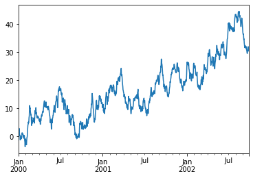
- 데이터프레임에서 plot() 메소드는 라벨이 존재하는 모든 열을 그릴 때 편리합니다.
1 | df = pd.DataFrame(np.random.randn(1000, 4), index=ts.index, |
<matplotlib.legend.Legend at 0x7f89eb792990>
<Figure size 432x288 with 0 Axes>
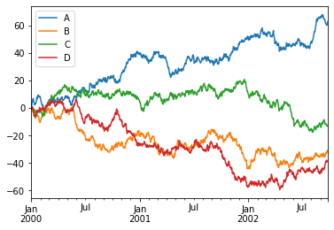
Getting Data In / Out (데이터 입출력)
CSV
- csv파일을 씁니다.
1 | df.to_csv('foo.csv') |
csv 파일을 읽습니다.
1 | pd.read_csv('foo.csv') |
| Unnamed: 0 | A | B | C | D | |
|---|---|---|---|---|---|
| 0 | 2000-01-01 | 0.077785 | 1.354574 | 0.335250 | -0.643291 |
| 1 | 2000-01-02 | 1.506306 | 0.603573 | 1.431830 | -0.151375 |
| 2 | 2000-01-03 | 2.046989 | -0.243843 | 1.469860 | -1.276268 |
| 3 | 2000-01-04 | 4.195420 | -0.137163 | 0.435910 | -1.063562 |
| 4 | 2000-01-05 | 5.022651 | -0.684153 | -0.179983 | 0.833490 |
| ... | ... | ... | ... | ... | ... |
| 995 | 2002-09-22 | 60.234084 | -33.177527 | -12.221695 | -38.068835 |
| 996 | 2002-09-23 | 60.599992 | -32.577022 | -13.140842 | -38.394246 |
| 997 | 2002-09-24 | 60.739624 | -30.809578 | -13.287040 | -38.570248 |
| 998 | 2002-09-25 | 60.622057 | -31.091125 | -13.027110 | -39.217957 |
| 999 | 2002-09-26 | 62.868526 | -31.140053 | -12.690182 | -39.383923 |
1000 rows × 5 columns
<script>
const buttonEl =
document.querySelector('#df-09d8c0d4-bf7c-472f-813c-05a5e4ad76fe button.colab-df-convert');
buttonEl.style.display =
google.colab.kernel.accessAllowed ? 'block' : 'none';
async function convertToInteractive(key) {
const element = document.querySelector('#df-09d8c0d4-bf7c-472f-813c-05a5e4ad76fe');
const dataTable =
await google.colab.kernel.invokeFunction('convertToInteractive',
[key], {});
if (!dataTable) return;
const docLinkHtml = 'Like what you see? Visit the ' +
'<a target="_blank" href=https://colab.research.google.com/notebooks/data_table.ipynb>data table notebook</a>'
+ ' to learn more about interactive tables.';
element.innerHTML = '';
dataTable['output_type'] = 'display_data';
await google.colab.output.renderOutput(dataTable, element);
const docLink = document.createElement('div');
docLink.innerHTML = docLinkHtml;
element.appendChild(docLink);
}
</script>
</div>
HDF5
- HDFStores에 읽고 씁니다.
- HDF5 Store에 씁니다.
1 | df.to_hdf('foo.h5', 'df') |
- HDF5 Store에서 읽어옵니다.
1 | pd.read_hdf('foo.h5', 'df') |
| A | B | C | D | |
|---|---|---|---|---|
| 2000-01-01 | 0.077785 | 1.354574 | 0.335250 | -0.643291 |
| 2000-01-02 | 1.506306 | 0.603573 | 1.431830 | -0.151375 |
| 2000-01-03 | 2.046989 | -0.243843 | 1.469860 | -1.276268 |
| 2000-01-04 | 4.195420 | -0.137163 | 0.435910 | -1.063562 |
| 2000-01-05 | 5.022651 | -0.684153 | -0.179983 | 0.833490 |
| ... | ... | ... | ... | ... |
| 2002-09-22 | 60.234084 | -33.177527 | -12.221695 | -38.068835 |
| 2002-09-23 | 60.599992 | -32.577022 | -13.140842 | -38.394246 |
| 2002-09-24 | 60.739624 | -30.809578 | -13.287040 | -38.570248 |
| 2002-09-25 | 60.622057 | -31.091125 | -13.027110 | -39.217957 |
| 2002-09-26 | 62.868526 | -31.140053 | -12.690182 | -39.383923 |
1000 rows × 4 columns
<script>
const buttonEl =
document.querySelector('#df-88b181fb-5386-46b5-93ff-12fa70dae0a4 button.colab-df-convert');
buttonEl.style.display =
google.colab.kernel.accessAllowed ? 'block' : 'none';
async function convertToInteractive(key) {
const element = document.querySelector('#df-88b181fb-5386-46b5-93ff-12fa70dae0a4');
const dataTable =
await google.colab.kernel.invokeFunction('convertToInteractive',
[key], {});
if (!dataTable) return;
const docLinkHtml = 'Like what you see? Visit the ' +
'<a target="_blank" href=https://colab.research.google.com/notebooks/data_table.ipynb>data table notebook</a>'
+ ' to learn more about interactive tables.';
element.innerHTML = '';
dataTable['output_type'] = 'display_data';
await google.colab.output.renderOutput(dataTable, element);
const docLink = document.createElement('div');
docLink.innerHTML = docLinkHtml;
element.appendChild(docLink);
}
</script>
</div>
Excel
- MS Excel에 읽고 씁니다.
- 엑셀 파일에 씁니다.
1 | df.to_excel('foo.xlsx', sheet_name='Sheet1') |
- 엑셀 파일을 읽어옵니다
1 | pd.read_excel('foo.xlsx', 'Sheet1', index_col=None, na_values=['NA']) |
| Unnamed: 0 | A | B | C | D | |
|---|---|---|---|---|---|
| 0 | 2000-01-01 | 0.077785 | 1.354574 | 0.335250 | -0.643291 |
| 1 | 2000-01-02 | 1.506306 | 0.603573 | 1.431830 | -0.151375 |
| 2 | 2000-01-03 | 2.046989 | -0.243843 | 1.469860 | -1.276268 |
| 3 | 2000-01-04 | 4.195420 | -0.137163 | 0.435910 | -1.063562 |
| 4 | 2000-01-05 | 5.022651 | -0.684153 | -0.179983 | 0.833490 |
| ... | ... | ... | ... | ... | ... |
| 995 | 2002-09-22 | 60.234084 | -33.177527 | -12.221695 | -38.068835 |
| 996 | 2002-09-23 | 60.599992 | -32.577022 | -13.140842 | -38.394246 |
| 997 | 2002-09-24 | 60.739624 | -30.809578 | -13.287040 | -38.570248 |
| 998 | 2002-09-25 | 60.622057 | -31.091125 | -13.027110 | -39.217957 |
| 999 | 2002-09-26 | 62.868526 | -31.140053 | -12.690182 | -39.383923 |
1000 rows × 5 columns
<script>
const buttonEl =
document.querySelector('#df-ceafdb00-9193-41c5-910f-15ff5b0d4b1b button.colab-df-convert');
buttonEl.style.display =
google.colab.kernel.accessAllowed ? 'block' : 'none';
async function convertToInteractive(key) {
const element = document.querySelector('#df-ceafdb00-9193-41c5-910f-15ff5b0d4b1b');
const dataTable =
await google.colab.kernel.invokeFunction('convertToInteractive',
[key], {});
if (!dataTable) return;
const docLinkHtml = 'Like what you see? Visit the ' +
'<a target="_blank" href=https://colab.research.google.com/notebooks/data_table.ipynb>data table notebook</a>'
+ ' to learn more about interactive tables.';
element.innerHTML = '';
dataTable['output_type'] = 'display_data';
await google.colab.output.renderOutput(dataTable, element);
const docLink = document.createElement('div');
docLink.innerHTML = docLinkHtml;
element.appendChild(docLink);
}
</script>
</div>
Gotchas (잡았다!)
- 연산 수행시 다음과 같은 예외 상황을 볼 수 도 있습니다.
- 이러한 경우에는 any(), all(), empty 등을 사용해서 무엇을 원하는지를 선택 (반영)해주어야 합니다.
1 | if pd.Series([False, True, False])is not None: |
I was not None true
Numpy 기초 문법
NumPy 기초 문법
NumPy 라이브 블러오기
1 | import numpy as np # 앨리어싱 |
1.21.5
배열로 변환
- 1부터 10까지의 리스트를 만든다.
- NumPy 배열로 변환해서 저장한다.
1 | temp = [1, 2, 3, 4, 5, 6, 7, 8, 9, 10] |
[ 1 2 3 4 5 6 7 8 9 10]
- 타입 확인하기
1 | print(type(temp)) |
<class 'list'>
<class 'numpy.ndarray'>
- arr 배열 숫자 5 출력
1 | print(arr[4]) # 인덱싱 |
5
[5 6 7 8]
- NumPy를 사용하여 기초 통계 함수를 사용한다.
1 | print(np.mean(arr)) # 평균 |
5.5
55
5.5
2.8722813232690143
사칙연산
1 | math_scores = [90, 80, 88] |
[90, 80, 88, 80, 70, 90]
1 | math_scores = [90, 80, 88] |
[170 150 178]
1 | print(np.min(total_scores)) # 최솟값 |
150
178
NumPy 메서드
사칙연산
1 | # 덧셈 |
덧셈: [170 150 178]
뺄셈: [10 10 -2]
곱셈: [7200 5600 7920]
나눗셈: [1.125 1.14285714 0.97777778]
거듭제곱: [0 0 0]
배열의 생성
- 0차원부터 3차원까지 생성하는 방법
- .shape 은 배열의 크기
- .ndim 은 차원을 알려준다.
1 | temp_arr = np.array(20) |
20
<class 'numpy.ndarray'>
()
0
1 | # 1차원 배열 |
[1 2 3]
<class 'numpy.ndarray'>
(3,)
1
2차원 배열
1 | temp_arr = np.array([[1, 2, 3],[4, 5, 6]]) |
[[1 2 3]
[4 5 6]]
<class 'numpy.ndarray'>
(2, 3)
2
3차원 배열
1 | temp_arr = np.array([[[1, 2, 3],[4, 5, 6]], [[1, 2, 3],[4, 5, 6]]]) |
[[[1 2 3]
[4 5 6]]
[[1 2 3]
[4 5 6]]]
<class 'numpy.ndarray'>
(2, 2, 3)
3
- 2 * 2 * 3 에서 각 숫자를 하나의 축이라고 생각하면 된다.
- 숫자가 3개니 3차원인 것이다.
1 | temp_arr = np.array([1, 2, 3, 4], ndmin = 2) |
[[1 2 3 4]]
<class 'numpy.ndarray'>
(1, 4)
2
- 마찬가지로, 1 * 4 는 2개의 축으로 이루어져 있으니 2차원인 것이다.
소숫점 정렬
1 | temp_arr = np.trunc([-1.23, 1,23]) |
array([-1., 1., 23.])
1 | temp_arr = np.fix([-1.23, 1,23]) |
array([-1., 1., 23.])
1 | temp_arr = np.around([-1.23789, 1,23789], 4) |
array([-1.2379e+00, 1.0000e+00, 2.3789e+04])
1 | temp_arr = np.round([-1.23, 1,23], 4) |
array([-1.23, 1. , 23. ])
1 | temp_arr = np.floor([-1.23, 1,23]) |
array([-2., 1., 23.])
1 | temp_arr = np.ceil([-1.23, 1,23]) |
array([-1., 1., 23.])
다양한 배열 생성 방법
1 | temp_arr = np.arange(5) # range |
array([0, 1, 2, 3, 4])
1 | temp_arr = np.arange(1, 9, 3) # 1에서부터 9까지 3칸씩 띄어라 |
array([1, 4, 7])
- np.zeros(()) 는 원하는 사이즈만큼 0으로 구성된 배열 생성
1 | zero_arr = np.zeros((2, 3)) # 원하는 사이즈만큼 0으로 구성된 배열 만들기 |
[[0. 0. 0.]
[0. 0. 0.]]
<class 'numpy.ndarray'>
(2, 3)
2
float64
flaot64, 이게 지금은 중요하지 않지만, 나중에 프로젝트를 할 때, 필요한 내용이다.
예를 들면, int32와 float64는 연산이 안된다.
np.ones(())는 원하는 사이즈만큼 1로 구성된 배열 생성
1 | temp_arr = np.ones((4, 5), dtype="int32") # 원하는 사이즈만큼 1로 구성된 배열 만들기 |
[[1 1 1 1 1]
[1 1 1 1 1]
[1 1 1 1 1]
[1 1 1 1 1]]
<class 'numpy.ndarray'>
(4, 5)
2
int32
reshape
- -1의 의미는 자동설정해준다는 것이다. 나중에 머신러닝할 때 유용하다.
- magic keyword라고 한다.
1 | temp_arr = np.ones((12, 12), dtype="int32") |
[[1 1 1 1 1 1 1 1 1 1 1 1 1 1 1 1 1 1 1 1 1 1 1 1 1 1 1 1 1 1 1 1 1 1 1 1]
[1 1 1 1 1 1 1 1 1 1 1 1 1 1 1 1 1 1 1 1 1 1 1 1 1 1 1 1 1 1 1 1 1 1 1 1]
[1 1 1 1 1 1 1 1 1 1 1 1 1 1 1 1 1 1 1 1 1 1 1 1 1 1 1 1 1 1 1 1 1 1 1 1]
[1 1 1 1 1 1 1 1 1 1 1 1 1 1 1 1 1 1 1 1 1 1 1 1 1 1 1 1 1 1 1 1 1 1 1 1]]
<class 'numpy.ndarray'>
(4, 36)
2
int32
numpy 조건식
np.where(조건식, 참, 거짓)
- 조건식이 하나일때 np.where()을 사용한다.
1 | temp_arr = np.arange(10) |
array([0, 1, 2, 3, 4, 5, 6, 7, 8, 9])
1 | # 5보다 작은 값은 원래값으로 반환 |
array([ 0, 1, 2, 3, 4, 50, 60, 70, 80, 90])
- 퀴즈
- 0 ~ 100 까지의 배열 생성 후, 50보다 작은 값은 곱하기 10, 나머지는 그냥 원래 값 반환
1 | temp_arr = np.arange(101) |
array([ 0, 10, 20, 30, 40, 50, 60, 70, 80, 90, 100, 110, 120,
130, 140, 150, 160, 170, 180, 190, 200, 210, 220, 230, 240, 250,
260, 270, 280, 290, 300, 310, 320, 330, 340, 350, 360, 370, 380,
390, 400, 410, 420, 430, 440, 450, 460, 470, 480, 490, 50, 51,
52, 53, 54, 55, 56, 57, 58, 59, 60, 61, 62, 63, 64,
65, 66, 67, 68, 69, 70, 71, 72, 73, 74, 75, 76, 77,
78, 79, 80, 81, 82, 83, 84, 85, 86, 87, 88, 89, 90,
91, 92, 93, 94, 95, 96, 97, 98, 99, 100])
np.select(condlist, choicelist, default = )
- 사실 다중조건을 더 많이 사용한다.
- 이 때는 np.select를 사용한다.
- condlist는 조건식 리스트이다.
- choicelist는 조건식이 참일때 수행할 명령 리스트이다.
- condlist와 choicelist 요소들은 맞춰주어야 한다.
- default를 설정 안해주면 0인데, 아래에서 확인해보자.
1 | temp_arr = np.arange(10) |
array([0, 1, 2, 3, 4, 5, 6, 7, 8, 9])
1 | condlist = [temp_arr > 5, temp_arr < 2] # 이거라면, |
[100 101 0 0 0 0 12 14 16 18]
[100 101 2 3 4 5 12 14 16 18]
교재 넘파이 부분 손코딩 실습
- 도미와 빙어를 분류하는 머신러닝 코드짜기
1 | fish_length = [25.4, 26.3, 26.5, 29.0, 29.0, 29.7, 29.7, 30.0, 30.0, 30.7, 31.0, 31.0, |
1 | from sklearn.neighbors import KNeighborsClassifier |
1 | print(fish_data[4]) # fish_data의 다섯 번째 샘플 가져오기 |
[29.0, 430.0]
1 | print(fish_data[0:5]) # fish_data의 처음 다섯 개의 샘플 가져오기 |
[[25.4, 242.0], [26.3, 290.0], [26.5, 340.0], [29.0, 363.0], [29.0, 430.0]]
1 | train_input = fish_data[:35] # 처음부터 34번째 인덱스까지는 훈련 세트 |
1 | kn = kn.fit(train_input, train_target) |
0.0
- 도미와 빙어가 골고루 섞여야 하는데 마지막 35번부터는 빙어만 있으니 제대로 학습을 못하게 된 것.
- 이것을 샘플링 편향 sampling bias
- 즉, 훈련 세트에 도미만 있기 때문에 테스트 세트가 무엇이든 도미로 판단하게 된다.
- 골고루 섞기 위해서 numpy 라이브러리가 필요하다.
1 | import numpy as np |
[[ 25.4 242. ]
[ 26.3 290. ]
[ 26.5 340. ]
[ 29. 363. ]
[ 29. 430. ]
[ 29.7 450. ]
[ 29.7 500. ]
[ 30. 390. ]
[ 30. 450. ]
[ 30.7 500. ]
[ 31. 475. ]
[ 31. 500. ]
[ 31.5 500. ]
[ 32. 340. ]
[ 32. 600. ]
[ 32. 600. ]
[ 33. 700. ]
[ 33. 700. ]
[ 33.5 610. ]
[ 33.5 650. ]
[ 34. 575. ]
[ 34. 685. ]
[ 34.5 620. ]
[ 35. 680. ]
[ 35. 700. ]
[ 35. 725. ]
[ 35. 720. ]
[ 36. 714. ]
[ 36. 850. ]
[ 37. 1000. ]
[ 38.5 920. ]
[ 38.5 955. ]
[ 39.5 925. ]
[ 41. 975. ]
[ 41. 950. ]
[ 9.8 6.7]
[ 10.5 7.5]
[ 10.6 7. ]
[ 11. 9.7]
[ 11.2 9.8]
[ 11.3 8.7]
[ 11.8 10. ]
[ 11.8 9.9]
[ 12. 9.8]
[ 12.2 12.2]
[ 12.4 13.4]
[ 13. 12.2]
[ 14.3 19.7]
[ 15. 19.9]]
1 | print(input_arr.shape) # shape 메서드로 배열 구성 확인. 49행 2열 |
(49, 2)
- 넘파이 배열로 준비는 마쳤다.
- 여기에서 랜덤으로 추출해보자.
- 아예 인덱스를 섞은 다음 input_arr와 target_arr에서 샘플을 선택하면 무작위로 훈련 세트를 나누는 셈이 될 것이다.
- 넘파이 arange() 함수를 사용해서 0부터 48까지 1씩 증가하는 인덱스를 만든다.
- 인덱스를 랜덤하게 섞는다.
- 넘파이에서 무작위 결과를 만드는 함수들은 실행할 때마다 다른 결과를 만들기 때문에 일정한 결과를 얻으려면 랜덤 시드(random seed)를 지정해줘야 한다.
1 | np.random.seed(42) # 일정한 결과를 얻기 위한 랜덤 시드(random seed) |
- 잘 만들어졌는지 체크해보자
1 | print(index) |
[13 45 47 44 17 27 26 25 31 19 12 4 34 8 3 6 40 41 46 15 9 16 24 33
30 0 43 32 5 29 11 36 1 21 2 37 35 23 39 10 22 18 48 20 7 42 14 28
38]
- 랜덤하게 섞인 인덱스를 가지고 전체 데이터를 훈련 세트와 테스트 세트로 나누자.
- 넘파이에 배열 인덱싱(array indexing) 기능 이용
1 | print(input_arr[[1,3]]) # input_arr 에서 두 번째와 네 번째 샘플 선택하여 추출 |
[[ 26.3 290. ]
[ 29. 363. ]]
- 랜덤하게 35개의 샘플을 훈련 세트로 만들기
1 | train_input = input_arr[index[:35]] |
- 만들어진 index의 첫 번째 값은 13임을 확인했다. 따라서, train_input의 첫 번째 원소는 input_arr의 열 네 번째 원소가 들어있을 것이다. 확인해보자.
1 | print(input_arr[13], train_input[0]) # 동일하다 |
[ 32. 340.] [ 32. 340.]
- 이번에는 나머지 14개를 테스트 세트로 만들자
1 | test_input = input_arr[index[35:]] |
- 데이터 세트들이 잘 섞였는 지 산점도 그래프로 확인
1 | import matplotlib.pyplot as plt |
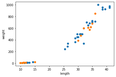
파이썬 기초 문법 3
클래스
클래스를 만드는 목적!
- 코드의 간결화
- 코드를 재사용
- 여러 라이브러리 –> 클래스로 구현이 됨
- list 클래스, str 클래스
- 객체로 씀
- 변수명으로 정의!
- 여러 클래스들이 모여서 하나의 라이브러리가 됨.
- 장고 / 웹개발 / 머신러닝 / 시각화/ 데이터 전처리
- 어렵다. 그러나 왜 쓰는지를 기억해야 한다. 모든 웹개발은 클래스로 구현된다. 지금 단계에서 클래스를 구현하는건 말도 안 된다.
1 | class Person: # class 대문자소문자소문자~: |
kim은 korean
lee은 korean
instance 메서드 생성
- list.appen(), list.extend()
1 | class Person: # class 대문자소문자소문자~: |
kim은 korean
lee은 korean
kim A을 노래합니다.
lee B을 노래합니다.
클래스 상속(inheritance)
- 부모님 유산…
- 부모님 집 (냉장고, 세탁기, TV, etc) # 부모 클래스 instance method, attribute
- 사용은 같이 함
- 여러분, 돈을 모음
- 개인 노트북 구매 ( 여러분 각자 방에 비치) # 자식 클래스 instance method, attribute 추가 확장
- 노트북은 내 거고, 추가 가전 제품을 구매해서 확장!
1 | class Parent: |
Child Class is ON
kim 현재 춤을 춥니다.
kim 연애을 노래합니다.
I am child
I am Parent!!
- AttributeError: ‘Parent’ object has no attribute ‘studying’
- Parent 클래스에 studying 속성이 없더라.
- 부모는 자식의 물건을 쓰지 않는다.
1 | class TV: |
Selling Price: 500
Selling Price: 500
Selling Price: 1000
클래스 내부에 조건문
- init constructor에 조건문을 써보자!
1 | class Employee: |
급여는 0원이 될 수 없다!. 다시 입력하셈!
hs
0
1500
4500
642.8571428571429
클래스 Docstring
1 | class Person: |
My name is Evan. I am 20 years old. 나의 직장은 00이야
Help on class Person in module __main__:
class Person(builtins.object)
| Person(name, age)
|
| 사람을 표현하는 클래스
|
| ...
|
| Attributes
| ----------
| name : str
| name of the person
|
| age : int
| age of the person
|
|
| Methods
| ----------
|
| info(additional=""):
| Prints the person's name and age
|
| Methods defined here:
|
| __init__(self, name, age)
| Constructs all the neccessary attributes for the person object
|
| Parameters
| ----------
| name : str
| name of the person
|
| age : int
| age of the person
|
| info(self, additional=None)
| 귀찮음...
|
|
| Parameters
| ----------
| additional : str, optional
| more info to be displayed (Default is None) / A, B, C
|
|
| Returns
| -------
| None
|
| ----------------------------------------------------------------------
| Data descriptors defined here:
|
| __dict__
| dictionary for instance variables (if defined)
|
| __weakref__
| list of weak references to the object (if defined)
파이썬 기초 문법 2
기초 문법 리뷰
1 | # 리스트 |
조건문 & 반복문
1 | if True: |
for문
for문의 기본 구조
1 | for 변수 in 리스트(또는 튜플, 문자열): |
전형적인 for문
1 | test_list = ['one', 'two', 'three'] |
one
two
three
다양한 for문의 사용
1 | a = [(1,2), (3,4), (5,6)] |
3
7
11
- 위 예는 a 리스트의 요솟값이 튜플이기 때문에 각각의 요소가 자동으로 변수에 대입된다.
for문의 응용
1 | marks = [90, 25, 67, 45, 80] |
1번 학생은 합격입니다.
2번 학생은 불합격입니다.
3번 학생은 합격입니다.
4번 학생은 불합격입니다.
5번 학생은 합격입니다.
for문과 continue
- while문 처럼 continue 사용가능하다. 즉 for문 맨 처음으로 돌아가게 된다.
1 | marks = [90, 25, 67, 45, 80] |
1번 학생 축하합니다. 합격입니다.
3번 학생 축하합니다. 합격입니다.
5번 학생 축하합니다. 합격입니다.
1 | for i in range(3): |
1 hel
2 hel
3 hel
1 | book_list = ["프로그래밍 R", "혼자 공부하는 머신러닝"] |
프로그래밍 R
혼자 공부하는 머신러닝
1 | strings01 = "Hello World" |
H
e
l
l
o
W
o
r
l
d
1 | num_tuple = (1, 2, 3, 4) # 튜플도 동일 |
1
2
3
4
1 | num_dict = {"A": 1, "B" : 2} # 딕셔너리는 뭔가 불안정 |
A
B
반복문의 필요성
1 | product_name = ["요구르트", "우유"] |
요구르트의 매출액은 5000원이다.
우유의 매출액은 4500원이다.
- 반복문이 필요하다!
1 | product_name = ["요구르트", "우유"] |
요구르트의 매출액은 5000원이다.
우유의 매출액은 4500원이다.
만약, 항목의 개수를 모른다면???
모르는게 생기면 구글링을 해야한다
구글 검색 엔진: how to count list in python
그렇게 해서 len함수를 찾아 냈다.
반복문을 바로 작성할 필요가 없다. 그러면 헷갈린다. 하나씩 직접해보고, 패턴을 발견하고, 그리고 짜는 것이다.
while문
- 얘도 반복문이다
- 조건식이 들어가는 것이 포인트(vs. for-loop는 정해진 범위가 포인트)
1 | count = 0 # 처음에 상수가 들어가야 한다. |
1 안녕하세요..
2 안녕하세요..
3 안녕하세요..
4 안녕하세요..
5 안녕하세요..
5를 초과했군요!
- 조건식이 만족할 때까지 계속 실행되다가 만족하지 않을 때 while문은 끝이 난다.
- 두 번째 방식 : 숫자를 차감하면서 반복하는 방식
1 | count = 3 |
2 안녕하세요..
1 안녕하세요..
0 안녕하세요..
0 미만 이군요!
“열 번 찍어 안 넘어가는 나무 없다”
1 | treeHit = 0 |
나무를 1번 찍었습니다.
나무를 2번 찍었습니다.
나무를 3번 찍었습니다.
나무를 4번 찍었습니다.
나무를 5번 찍었습니다.
나무를 6번 찍었습니다.
나무를 7번 찍었습니다.
나무를 8번 찍었습니다.
나무를 9번 찍었습니다.
나무를 10번 찍었습니다.
나무 넘어갑니다.
while문 강제로 빠져나가기(break)
- 커피 자판기 예
1 | coffee = 10 |
돈을 받았으니 커피를 줍니다.
남은 커피의 양은 9개입니다.
돈을 받았으니 커피를 줍니다.
남은 커피의 양은 8개입니다.
돈을 받았으니 커피를 줍니다.
남은 커피의 양은 7개입니다.
돈을 받았으니 커피를 줍니다.
남은 커피의 양은 6개입니다.
돈을 받았으니 커피를 줍니다.
남은 커피의 양은 5개입니다.
돈을 받았으니 커피를 줍니다.
남은 커피의 양은 4개입니다.
돈을 받았으니 커피를 줍니다.
남은 커피의 양은 3개입니다.
돈을 받았으니 커피를 줍니다.
남은 커피의 양은 2개입니다.
돈을 받았으니 커피를 줍니다.
남은 커피의 양은 1개입니다.
돈을 받았으니 커피를 줍니다.
남은 커피의 양은 0개입니다.
커피가 다 떨어졌습니다. 판매를 중지합니다.
while문의 맨 처음으로 돌아가기(continue)
1 | a = 0 |
1
3
5
7
9
continue는 while문 맨 처음으로 돌아가게 한다.(조건문: a<10)
개발자를 지향한다면, while문 공부를 좀 더 비중있게 다루는 게 좋다.
데이터 분석가를 지향한다면, while문을 쓸 일이 별로 없다. for-loop 공부를 좀 더 비중있게 하는 게 좋다.
사용자 정의 함수 (User-Defined Function)
- 이거 왜 쓸까?
클래스(Class)를 왜 쓸까?
- 코드의 반복성을 줄이기 위해서 사용하는 것이다.
len() —> 누군가가 만들었고, 우리는 그걸 그냥 쓰는 것이다.
- 리스트의 길이 구할 때 쓴다.
- 리스트의 전체 길이를 구하겠다!? -> 1회성? 나만 쓰는가?
1 | def 함수명(): |
1 | # 더하기 함수 만들기 |
3
1 | # 빼기 함수 만들기 |
-1
1 | # 곱하기 함수 만들기 |
2
1 | # 나누기 함수 만들기 |
0.5
jupyter notebook, .ipynb 확장자명
.py로 저장 (pycharm..)
- basic.py로 저장할 때, 예시
1 | # /user/local/bin/python |
파이썬 함수 주석 처리
- docstring 작업
- 나중에 프로젝트할 때 필요할 것이다.
- 코드 작성 마지막 단계에서 필히 추가해야할 내용이다.
1 | # /user/local/bin/python |
Help on function temp in module __main__:
temp(content, letter)
content안에 있는 문자를 세는 함수입니다.
Args:
content(str) : 탐색 문자열
letter(str) : 찾을 문자열
Returns:
int
리스트 컴프리헨션
- for-loop를 한 줄로 처리
- 리스트 안에 for-loop를 쓸 수 있다.
- 어렵다.
1 | my_list = [[10], [20, 30]] |
10
20
30
[10, 20, 30]
1 | my_list = [[10], [20, 30]] |
[10, 20, 30]
1 | # 다른 예제 |
['h', 'e', 'l', 'l', 'o', 'w', 'o', 'r', 'l', 'd']
1 | letters2 = [char for char in "helloworld"] |
['h', 'e', 'l', 'l', 'o', 'w', 'o', 'r', 'l', 'd']
사용자 정의 함수 다시
1 | def mean_and_median(value_list): |
avg: 2.5714285714285716
median: 2
- 데코레이터, 변수명 immutable or mutable, context manager 등의 내용은 점프 투 파이썬에 없다. 파이썬 코딩 도장에 있다.
파이썬 기초 문법
Hello World
1 | print("Hello, World!") |
Hello, World!
주석 처리
- 코드 작업 시, 특정 코드에 대해 설명
- 사용자 정의 함수 작성 시, 클래스 작성 시..(도움말 작성..)
1 | # 한 줄 주석 처리 |
Hello
변수 ( Scalar)
- 객체(object)로 구현이 됨
- 하나의 자료형(Type)을 가진다. (이것만 기억!)
- 클래스로 정의가 됨.
- 다양한 함수들이 존재 함.
int
- int 정수를 표현하는 데 사용함.
1 | # 데이터 전처리... |
1
<class 'int'>
float
- 실수를 표현하는데 사용한다.
1 | num_float = 0.2 |
0.2
<class 'float'>
bool
- True와 False로 나타내는 Boolean 값을 표현하는 데 사용한다.
1 | bool_true = True |
True
<class 'bool'>
None
- Null을 나타내는 자료형으로 None이라는 한 가지 값만 가집니다.
1 | none_x = None |
None
<class 'NoneType'>
사칙연산
- 정수형 사칙 연산
1 | a = 13 |
a + b = 60
-34
611
0.2765957446808511
0
13
22664052024539238871968220999332552715703774239747717
실수형 사칙연산
1 | a = 13.0 |
a + b = 60.0
-34.0
611.0
0.2765957446808511
0.0
13.0
2.2664052024539239e+52
논리형 연산자
- Bool 형은 True와 False 값으로 정의
- AND / OR
1 | x = 5 > 4 |
True
False
False
False
----
True
True
True
False
비교 연산자
- 부등호를 의미합니다.
- 비교 연산자를 True와 False값을 도출
논리 & 비교 연산자 응용
1 | var = input("입력하여 주세요..") |
입력하여 주세요123
<class 'str'>
- input은 문자열로 만들어버린다.
- 형변환을 해준다.
- 문자열, 정수, 실수 등등등
1 | var = int("1") |
<class 'int'>
1 | var = int(input("숫자를 입력하여 주세요")) |
숫자를 입력하여 주세요12345
<class 'int'>
1 | num1 = int(input("숫자를 입력하여 주세요...")) # 10 |
숫자를 입력하여 주세요...10
숫자를 입력하여 주세요...3
숫자를 입력하여 주세요...5
숫자를 입력하여 주세요...7
True
True
변수 (Non Scalar)
- 문자열을 입력
1 | print("'Hello, World!'") |
'Hello, World!'
"Hello, World!"
1 | print("Hello world") |
Hello world
- 섞이면 안 된다.
string 연산자
- 덧셈 연산자를 써보자.
1 | str1 = "Hello " |
Hello World!
- 곱셈 연산자를 사용해본다.
1 | greeting = str1 + str2 |
Hello World! Hello World! Hello World! Hello World!
Indexing
- 문자열 인덱싱은 각각의 문자열 안에서 범위를 지정하여 특정 문자를 추출한다.
1 | greeting = "Hello Kaggle!" |
K
l
- 0부터 시작해서 6번째가 “K”이다. 공백도 포함해서
슬라이싱
- 범위를 지정하고 데이터를 가져온다.
1 | greeting |
Hello Kaggle!
Kaggle!
Hello
lo Ka
HloKg
1 | # greeting[13] # 스트링 인덱스가 범위 밖에 있다는 에러 메세지 |
문자열을 바꾸려면
- 바꾸고 싶은 부분을 기준으로 나누고 원하는 문자를 삽입한다.
1 | a = "pithon" |
'python'
문자열 포매팅
- 문자열 안의 특정한 값을 바꿔야 할 경우가 있을 때 사용하는 기법.
1 | "I eat %d apples." % 3 |
'I eat five apples.'
1 | "I eat %s apples." % "five" |
'I eat five apples.'
- 숫자를 넣기 위해서는 %d
- 문자열을 넣기 위해서는 %s
1 | number = 3 |
'I eat 3 apples.'
- 숫자를 바로 대입하나 위 처럼 숫자 값을 나타내는 변수를 대입하나 결과는 같다.
1 | number = 10 |
'I ate 10 apples. so I was sick for three days.'
위 처럼 2개 이상의 값을 넣으려면 마지막 % 다음 괄호 안에 콤마로 구분하여 각각의 값을 넣어 주면 된다.
문자열 포맷 코드
- 정수와 문자열 외에도 다양한 것을 대이할 수 있다.
- %s 는 문자열
- %c 는 문자 1개(character)
- %d 는 정수(integer)
- %f 는 부동소수(floating-point)
- %o 는 8진수
- %x 는 16진수
- %% 는 Literal % (문자 % 자체)
1 | "I have %s apples." % 3 |
'I have 3 apples.'
1 | "rate is %s" % 2.345 |
'rate is 2.345'
- 흥미롭게도 %s 포맷 코드는 어떤 형태의 값이든 변환해 넣을 수 있다. 왜냐하면 % 뒤에 있는 값을 문자열로 바꾸기 때문이다.
포매팅 연산자 %d와 %를 같이 쓸때는 %%를 쓴다.
1 | "Error is %d%%." % 98 |
'Error is 98%.'
포맷 코드와 숫자 함께 사용하기
- 포맷 코드를 숫자와 함께 사용하면 더욱 유용하다
- 정렬과 공백
1 | "%10s" % "hi" |
' hi'
- %10s는 전체 길이가 10개인 문자열 공간에서 대입되는 값을 오른쪽으로 정렬하고 그 앞의 나머지는 공백으로 남겨 두라는 의미다.
1 | "%-10sjane" % 'hi' |
'hi jane'
- hi를 왼쪽으로 정렬하고 나머지는 공백으로 채웠음을 볼 수 있다.
- 소수점 표현하기
1 | "%0.4f" % 3.42134234 |
'3.4213'
- 3.42134234를 소수점 네 번째 자리까지만 나타내고 싶은 경우에는 위와 같이 사용한다. ‘.’ 뒤의 숫자 4는 소수점 뒤에 나올 숫자의 개수를 의미한다.
1 | "%10.4f" %3.42134234 |
' 3.4213'
- 위 예는 숫자 3.42134234를 소수점 네 번째 자리까지만 표시하고 전체 길이가 10개인 문자열 공간에서 오른쪽으로 정렬하는 예를 보여준다.
format 함수를 사용한 포맷팅
- 문자열의 format 함수를 사용하면 좀 더 발전된 스타일로 문자열 포맷을 지정할 수 있다.
1 | "I eat {0} apples".format(3) |
'I eat 3 apples'
- {0} 부분이 숫자 3으로 바뀌었다.
1 | number = 3 |
'I eat 3 apples'
- {0} 항목이 number 변수 값인 3으로 바뀌었다.
1 | number = 10 |
'I ate 10 apples. so I was sick for three days.'
- 2개 이상의 값을 넣을 경우 문자열의 {0}, {1}과 같은 인덱스 항목이 format 함수의 입력값으로 순서에 맞게 바뀐다.
1 | "I ate {number} apples. so I was sick for {day} days.".format(number=10, day=3) |
'I ate 10 apples. so I was sick for 3 days.'
- name=value와 같은 형태의 입력값이 있어야만 한다.
1 | "I ate {0} apples. so I was sick for {day} days.".format(10, day=3) |
'I ate 10 apples. so I was sick for 3 days.'
- 위와 같이 인덱스 항목과 name=value 형태를 혼용하는 것도 가능하다.
1 | "{0:<10}".format("hi") |
'hi '
- :<10 표현식을 사용하면 치환되는 문자열을 왼쪽으로 정렬하고 문자열의 총 자릿수를 10으로 맞출 수 있다.
1 | "{0:>10}".format("hi") |
' hi'
- 위 예문은 오른쪽 정렬
1 | "{0:^10}".format("hi") |
' hi '
- 가운데 정렬은 :^ 기호를 사용한다.
1 | "{0:=^10}".format("hi") |
'====hi===='
- 정렬할 때 공백 대신 지정한 문자 값으로 채워 넣는 것도 가능하다. 채워 넣을 문자 값은 정렬 문자 <, >, ^ 바로 앞에 넣어야 한다.
1 | "{0:!<10}".format("hi") |
'hi!!!!!!!!'
1 | y = 3.42134234 |
'3.4213'
- 위 예는 format 함수를 사용해 소수점을 4자리까지만 표현하는 방법을 보여 준다.
1 | "{0:10.4f}".format(y) |
' 3.4213'
- 위 예는 자릿수를 10으로 맞춰준 것이다.
f 문자열 포매팅
- 다음과 같이 문자열 앞에 f 접두사를 붙이면 f 문자열 포매팅 기능을 사용할 수 있다.
- f 문자열 포매팅은 표현식(변수와 +, -같은 수식을 함께 사용하는 것)을 지원한다.
1 | name = '홍길동' |
'나의 이름은 홍길동입니다. 나이는 30입니다.'
1 | age = 30 |
'나는 내년이면 31살이 된다.'
- 딕셔너리는 f 문자열 포매팅에서 다음과 같이 사용할 수 있다.
1 | d = {'name':'홍길동', 'age':30} |
'나의 이름은 홍길동입니다. 나이는 30입니다.'
- 정렬은 다음과 같이 할 수 있다.
1 | f'{"hi":<10}' #왼쪽 정렬 |
' hi '
- 공백 채우기
1 | f'{"hi":=^10}' |
'====hi===='
- 소수점 표현
1 | y = 3.42134234 |
'3.4213'
문자열 관련 함수들
- 문자열 내장 함수
count함수
- 문자 개수 세기
1 | a = "hobby" |
2
find함수
- 위치 알려주기1
1 | a = "python is the best choice" |
-1
- 문자열 중 문자 b가 처음으로 나온 위치가 14라는 뜻
- 만약 k처럼 문자가 없으면 -1을 반환한다.
index함수
- 위치 알려주기2
1 | a = "Life is too short" |
8
- find함수와 마찬가지로 문자 t가 맨 처음으로 나온 위치를 반환한다.
- 만약 찾는 문자열이 존재하지 않는다면 오류를 발생시킨다.
join 함수
- 문자열 삽입
1 | ",".join('abcd') |
'a,b,c,d'
- abcd 문자열의 각각 ‘,’를 삽입한다.
upper 함수 / lower 함수
- 소문자를 대문자로 바꾸기
- 대문자를 소문자로 바꾸기
1 | a = "hi" |
'HI'
lstrip 함수 / rstrip 함수 / strip 함수
- 왼쪽 공백 지우기
- 오른쪽 공백 지우기
- 양쪽 공백 지우기
1 | a = " hi " |
'hi '
replace 함수
- 문자열 바꾸기
1 | a = "Life is too short" |
'Your leg is too short'
split 함수
- 문자열 나누기
1 | a = "Life is too short" |
['a', 'b', 'c', 'd']
- a.split() 처럼 괄호안에 아무 값도 넣어 주지 않으면 공백을 기준으로 문자열을 나눈다.
- 만약 b.split(‘:’) 처럼 괄호 안에 특정 값이 있을 경우에는 그걸 구분자로 한다.
리스트
- 시퀀스 데이터 타입
- 데이터에 순서가 존재하냐! 슬라이싱이 가능해야 함.
- 대괄호(‘[값1, 값2, 값3]’)
1 | a = [] # 빈 리스트 생성 |
[]
[]
[1]
['apple']
[1, 2, ['apple']]
<class 'list'>
리스트 슬라이싱
1 | a = [1, 2, 3, 4, 5, 6, 7, 8, 9, 10] |
1
[7, 8, 9, 10]
[1, 2, 3, 4, 5]
[4, 5]
[5, 6, 7]
[3, 4, 5, 6, 7, 8]
[2, 5, 8]
1 | a = [["apple", "banana", "cherry"], 1] # 중첩 리스트 |
['apple', 'banana', 'cherry']
banana
e
e
e
e
1 | a = [1, 2, 3, 4, 5, 6, 7, 8, 9, 10] |
[10, 9, 8, 7, 6, 5, 4, 3, 2, 1]
[1, 3, 5, 7, 9]
리스트 연산자
1 | a = ["john", "evan"] |
['john', 'evan', 'alice', 'sarah']
['alice', 'sarah', 'john', 'evan']
1 | c = a * 3 |
a * 3 = ['john', 'evan', 'john', 'evan', 'john', 'evan']
b * 0 = []
리스트 길이 구하기
- 리스트 길이를 구하기 위해서는 len 함수를 사용한다
1 | a = [1, 2, 3] |
3
리스트 수정 및 삭제
1 | a = [0, 1, 2] |
[0, 'b', 2]
리스트 값 추가하기
1 | a = [100, 200, 300] |
[100, 200, 300, 400]
- a를 저장해주지 않았는데도 append메서드를 사용했더니 자동저장되었다. 파이썬에 이런게 은근 많다. 모두 알려고 하지 말고 만나는대로 습득하는 수밖에 없다.
1 | a.append([500, 600]) |
[100, 200, 300, 400, [500, 600]]
1 | a = [100, 200, 300] |
[100, 200, 300, 500, 600]
1 | a = [ 0, 1, 2] |
[0, 100, 1, 2]
리스트 값 삭제하기
1 | a = [4, 3, 2, 1, "A"] |
[4, 3, 2, 'A']
[4, 3, 2]
1 | a = [1, 2, 3, 4, 5, 6, 7, 8, 9, 10] |
[1, 3, 4, 5, 6, 7, 8, 9, 10]
[1, 7, 8, 9, 10]
pop 함수
- 리스트의 맨 마지막 요소를 돌려주고 그 요소는 삭제한다.
1 | b = ["a", "b", "c", "d"] |
d
['a', 'b', 'c']
그 외 메서드
1 | a = [0, 1, 2, 3] |
[0, 1, 2, 3]
[]
1 | a = ["a", "a", "b", "b"] |
0
2
1 | a = [1, 4, 5, 2, 3] |
sort(): [1, 2, 3, 4, 5]
sort(reverse=True): [5, 4, 3, 2, 1]
- 내림차순 같은 옵션을 알아내는 방법은 구글링이다.
1 | c = [4, 3, 2, 'a'] |
reverse 함수
- 리스트 뒤집기
- 리스트를 역순으로
1 | a = ['a', 'b', 'c'] |
['c', 'b', 'a']
index 함수
- 위치 반환
1 | a = [1, 2, 3] |
2
extend
- 리스트 확장
- extend(x)에서 x에는 리스트만 올 수 있다.
- a.extend([4, 5])는 a += [4, 5]와 동일하다.
1 | a = [1, 2, 3] |
[1, 2, 3, 4, 5]
[1, 2, 3, 4, 5, 6, 7]
튜플
- List와 비슷하다.
- 슬라이싱, 인덱싱 등등
- (vs 리스트) : 튜플은 수정 삭제가 안된다.
1 | tuple1 = (0) # 끝에 콤마(,)를 붙이지 않을 때 --> int |
<class 'int'>
<class 'tuple'>
<class 'tuple'>
1 | a = (0, 1, 2, 3, 'a') |
<class 'tuple'>
튜플 인덱싱 및 슬라이싱 하기
1 | a = (0, 1, 2, 3, 'a') |
1
3
a
더하기 곱셈 연산자 사용
1 | t1 = (0, 1, 2, 3) |
(0, 1, 2, 3, 4, 5, 6, 7)
(0, 1, 2, 3, 0, 1, 2, 3, 0, 1, 2, 3)
()
딕셔너리
- key-value값으로 나뉨.
1 | dict_01 = {'teacher' : 'evan', |
{'teacher': 'evan', 'class': 601, 'student': 24, '학생이름': ['A', 'Z']}
evan
601
['A', 'Z']
1 | print(dict_01.keys()) |
dict_keys(['teacher', 'class', 'student', '학생이름'])
1 | print(dict_01.values()) |
dict_values(['evan', 601, 24, ['A', 'Z']])
1 | dict_01.items() # 튜플 형태로 묶이더라 |
dict_items([('teacher', 'evan'), ('class', 601), ('student', 24), ('학생이름', ['A', 'Z'])])
1 | print(dict_01.get("teacher")) # get메서드 |
evan
None
601
None
없어용
조건문 & 반복문
조건문
- 일상에서 조건문 언제쓸까요?
1 | weather = "비" |
우산을 가져간다.
- 등급표를 만들어보자
- 60점 이상 합격 / 그외는 불합격
- 숫자는 아무거나 써도 상관없음
1 | score = 61 |
합격
1 | score = int(input("점수를 입력하세요...")) # input은 문자열로 인식을 하니까 정수형으로 형변환 |
점수를 입력하세요...70
합격
- 등급으로 나눠보자
- 90점 이상은 A등급
- 80점 이상은 B등급
- 나머지는 F등급
- if-elif-else
1 | score = int(input("점수를 입력해 주세요: ")) |
점수를 입력해 주세요: 95
A등급
반복문
- 안녕하세요! 10번 반복하세요.
1 | print("안녕하세요!") |
- 2번째 과제 : 안녕하세요! 789256번 반복하세요.
1 | # 789... 뭐시기 반복하기 |
1 안녕하세요!
2 안녕하세요!
3 안녕하세요!
1 | count = range(3) |
range(0, 3)
0
1
2
1 | count = range(50) |
range(0, 50)
1번째
슈팅
2번째
슈팅
3번째
슈팅
4번째
슈팅
5번째
그만
1 | a = "hello" |
h
e
- 반복문 작성 방식은 다양하다.
- zip, range, enumerate, len 등등
1 | alphabets = ['A', 'B', 'c'] |
0 A
1 B
2 c